Model Interpretation and Feature Selection

10/28/2022

Robert Utterback (based on slides by Andreas Muller)

\( \renewcommand{\vec}[1]{\boldsymbol{#1}} \newcommand{\E}{\mathop{\boldsymbol{E}}} \newcommand{\var}{\boldsymbol{Var}} \newcommand{\norm}[1]{\lvert\lvert#1\rvert\rvert} \newcommand{\abs}[1]{\lvert#1\rvert} \newcommand{\ltwo}[1]{\norm{#1}_2} \newcommand{\lone}[1]{\norm{#1}_1} \newcommand{\sgn}[1]{\text{sign}\left( #1 \right)} \newcommand{\e}{\mathrm{e}} \newcommand{\minw}{\min_{\vec{w} \in \mathbb{R}^p, b\in\mathbb{R}}} \newcommand{\summ}{\sum_{i=1}^m} \newcommand{\sumn}{\sum_{i=1}^n} \newcommand{\logloss}{\ln{(\exp{(-y^{(i)}(\vec{w}^T\vec{x}^{(i)}+b))} + 1)}} \newcommand{\ai}{\alpha^{(i)}} \newcommand{\w}{\vec{w}} \newcommand{\wt}{\vec{w}^T} \newcommand{\xi}{\vec{x}^{(i)}} \newcommand{\xit}{(\vec{x}^{(i)})^T} \newcommand{\xip}{\xit \vec{w}} \newcommand{\tip}{(\phi(\xi)^T \phi(\vec{x}))} \)

Model Interpretation (post-hoc?)

NOT causal inference

Does x cause y?
That's NOT what model interpretation is giving us!
Don't want to get too into 'causal inference', but just be careful
Can still inform how to better model the data or do better exploration

Types of explanations

Explain model globally

How does the output depend on the input? Often: some form of 'marginals'

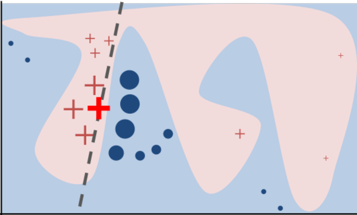
Explain model locally

Why does it classify this point this way?
Explanation could look like a 'global' one but be different for each point
"What is the minimum change to classify it differently?"

Explaining the model \(\ne\) explaining the data

model inspection only tells you about the model
the model might not accurately reflect the data

"Features important to the model"?

Naive:

coef_ for linear models
feature_importances_ for tree-based models

Linear Model coefficients

Relative importance only meaningful after scaling
Correlation among features might make coefficients completely uninterpretable
L1 regularization will pick one at random from a correlated group
Any penalty will invalidate usual interpretation of linear coefficients

Drop Feature Importance

\[ I^{drop}_i = Acc(f,X,y) - Acc(f',X_{-i},y) \]

def drop_feature_importance(est, X, y):
    base_score = np.mean(cross_val_score(est, X, y))
    scores = []
    for feature in range(X.shape[1]):
        mask = np.ones(X.shape[1], 'bool')
        mask[feature] = False
        X_new = X[:, mask]
        this_score = np.mean(cross_val_score(est, X_new, y))
        scores.append(base_score - this_score)
    return np.array(scores)

Doesn't really explain model (refits for each features
Can't deal with correlated features well
Very slow
Can be used for feature selection

Permutation Importance

Idea: measure marginal influence of one feature \[ I^{perm}_i = Acc(f,X,y) - E_{x_i}[Acc(f(x_i,X_{-i}),y)] \]

def permutation_importance(est, X, y, n_repeat=100):
  baseline_score = estimator.score(X, y)
  for f_idx in range(X.shape[1]):
      for repeat in range(n_repeat):
          X_new = X.copy()
          X_new[:, f_idx] = np.random.shuffle(X[:, f_idx])
          feature_score = estimator.score(X_new, y)
          scores[f_idx, repeat] = baseline_score - feature_score

Applied on a validation set given trained estimator.
Also kind of slow.

LIME

Build sparse linear local model around each data point
Explain prediction for each point locally
Paper: "Why Should I Trust Y ou" explaining the predictions of any classifier
Implementation: https://github.com/marcotcr/lime

SHAP

Build around idea of Shapley values
Roughly: does drop-out importance for every subset of features
Intractable, requires sample approximations
Fast variants for linear and tree-based models
Cool visualizations and tools: https://github.com/slundberg/shap
Can give local and global explanations

Case Study

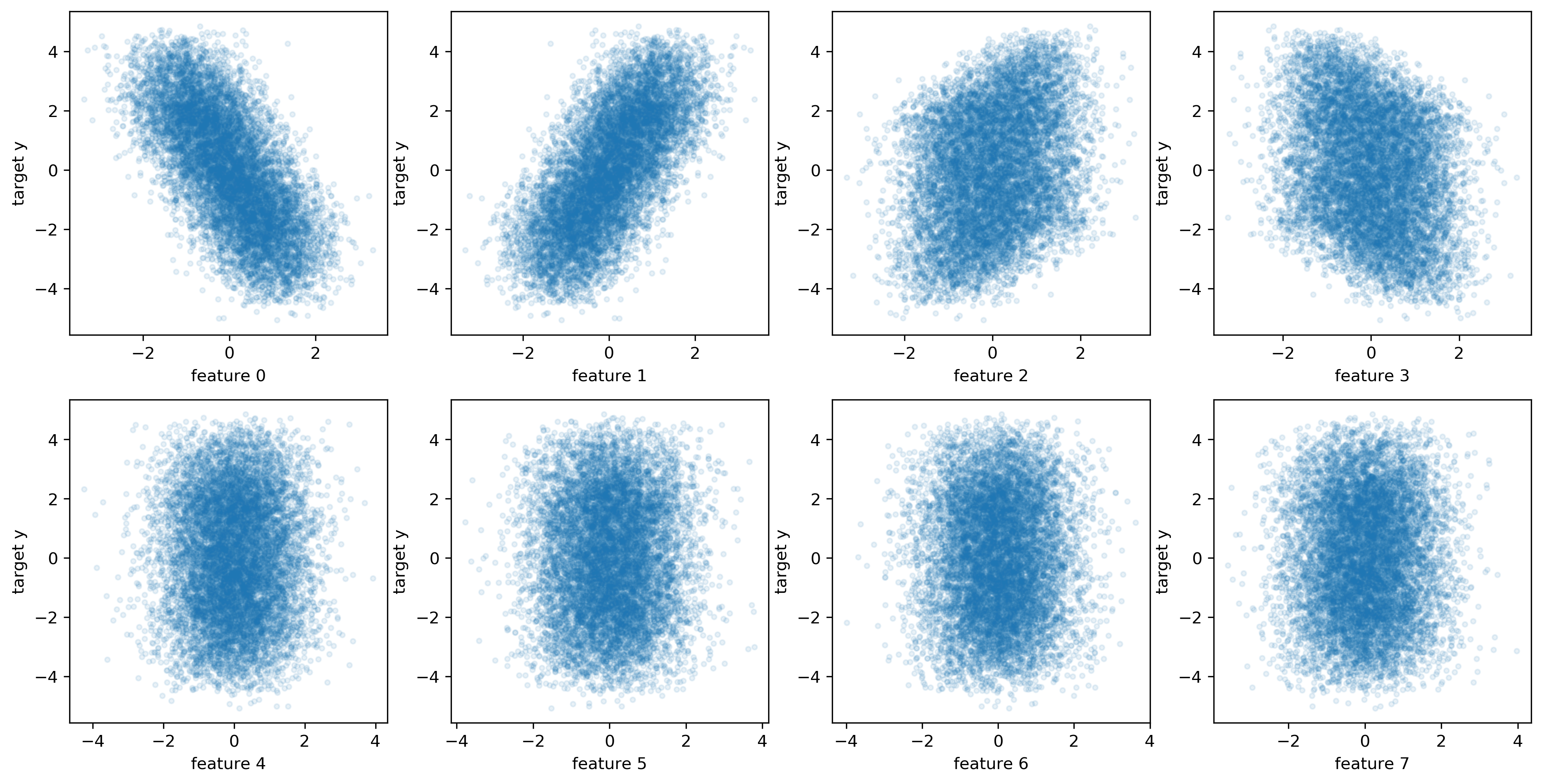
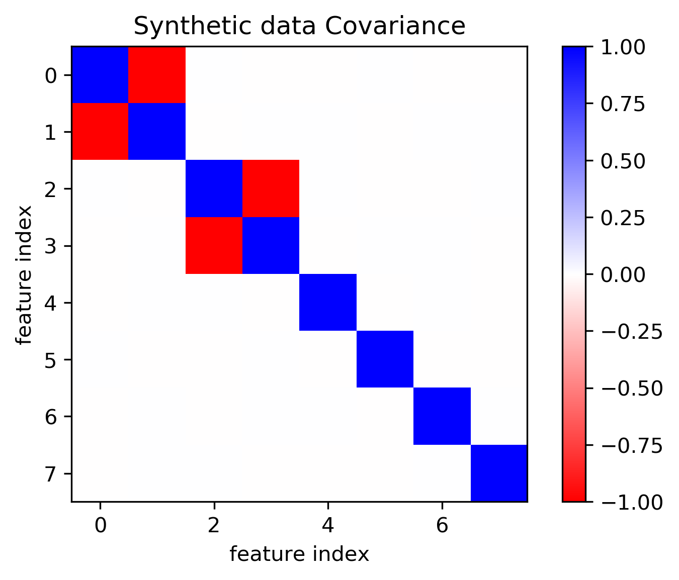
Toy Data

100,000 points, 8 features

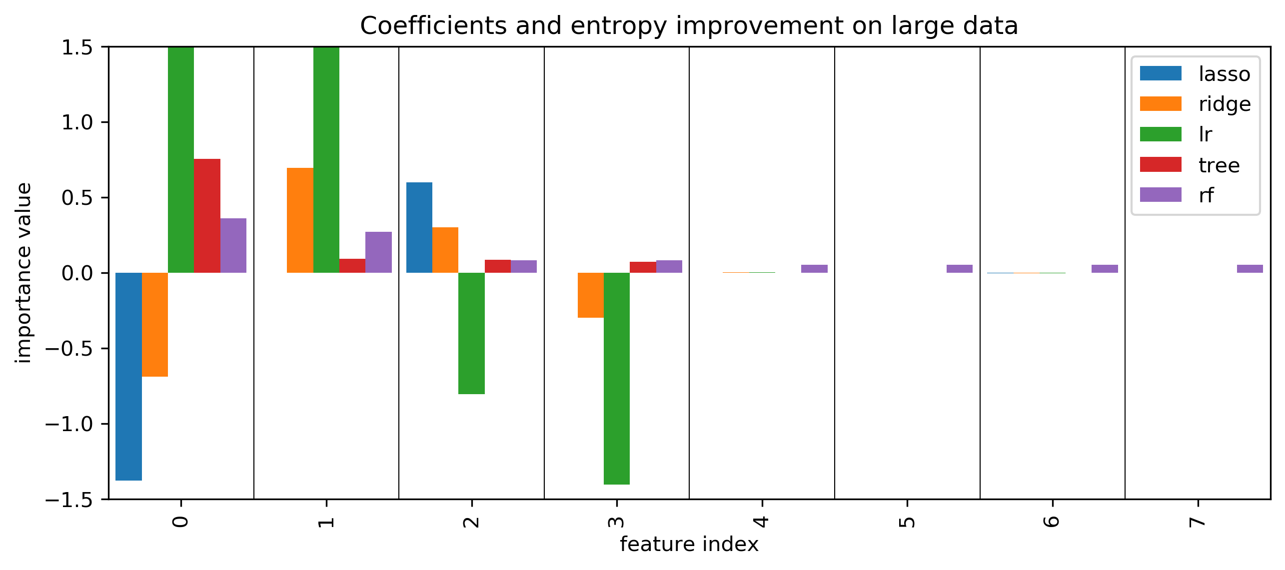
Models on lots of data

lasso = LassoCV().fit(X_train, y_train)
lasso.score(X_test, y_test)

0.545

ridge = RidgeCV().fit(X_train, y_train)
ridge.score(X_test, y_test)

0.545

lr = LinearRegression().fit(X_train, y_train)
lr.score(X_test, y_test)

0.545

param_grid = {'max_leaf_nodes': range(5, 40, 5)}
grid = GridSearchCV(DecisionTreeRegressor(), param_grid, cv=10, n_jobs=3)
grid.fit(X_train, y_train)
grid.score(X_test, y_test)

0.545

rf = RandomForestRegressor(min_samples_leaf=5).fit(X_train, y_train)
rf.score(X_test, y_test)

0.542

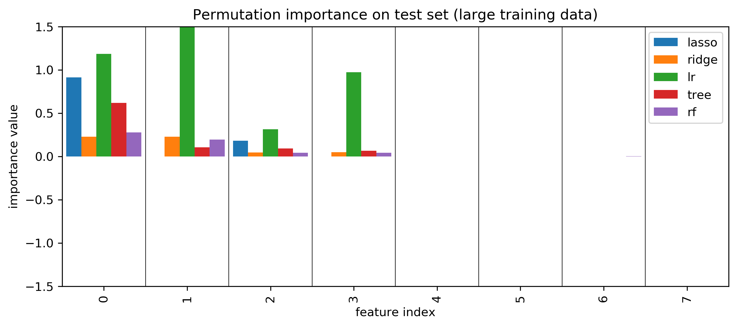
Coefficients and default feature importance

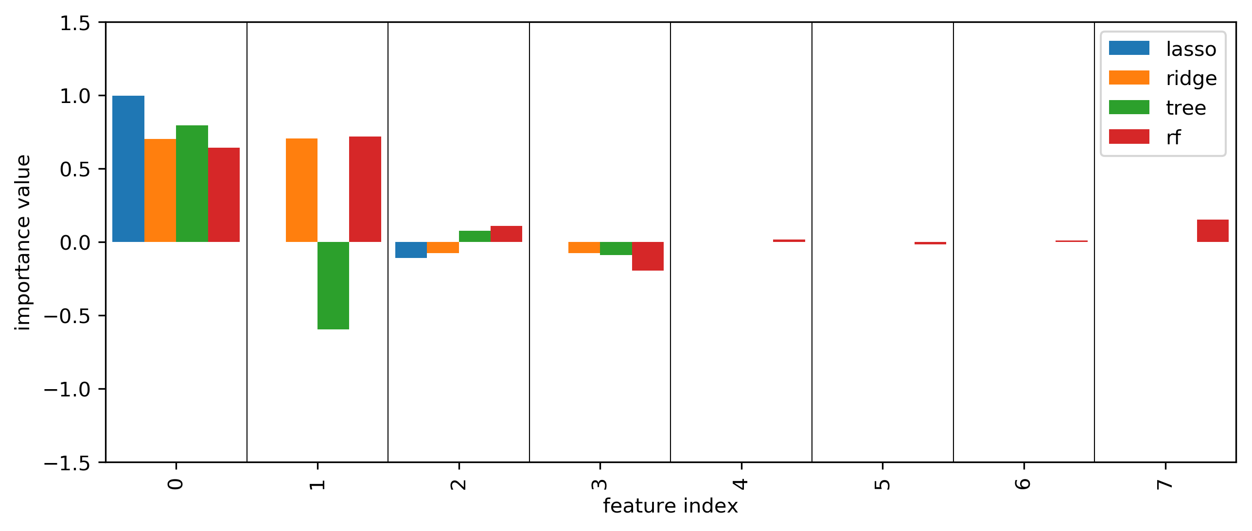
Permutation Importances

SHAP values

More model inspection

Kind of coarse-grained: just tells you how important
How about telling us exactly how a feature interacts with a given model/prediction

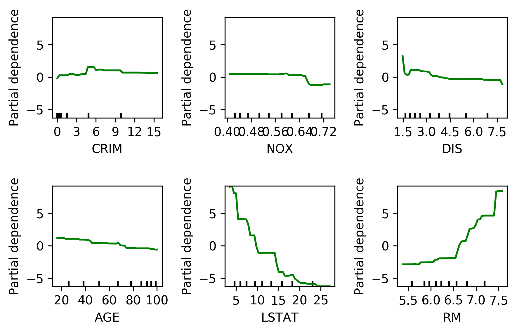
Partial Dependence plots

Marginal dependence of prediction on one (or two) features \[ f^{pdp}_i(x_i) = E_{X_{-i}}[f(x_i,x_{-i})] \]
Idea: get marginal predictions given feature
How? "integrate out" other features using validation data
Fast methods available for tree-based models (doesn't require validation data)

Partial Dependence

from sklearn.ensemble.partial_dependence import plot_partial_dependence
boston = load_boston()
X_train, X_test, y_train, y_test = \
    train_test_split(boston.data, boston.target,
                     random_state=0)

gbrt = GradientBoostingRegressor().fit(X_train, y_train)

fig, axs = \
    plot_partial_dependence(gbrt, X_train,
                            np.argsort(gbrt.feature_importances_)[-6:],
                            feature_names=boston.feature_names, n_jobs=3,
                            grid_resolution=50)

But there's also something else that's quite interesting, which is called Partial Dependence Plots that's actually possible for all trees. Unfortunately, in scikit-learn, it’s available only for the gradient boosting. So the idea here is to not only see what parameters are important but how will they influence the target. And so after you fit your model, I'm using the Boston data set to the gradient boosting regressor, there's a thing called plot partial dependence, which gets the model and the training data set and then the features for which I want to make the partial dependence plots.

For trees, don't actually need validation set (but in general you do!)
Trees actually have a faster way that doesn't require the brute force
Plots shown backwards (RM is most important)
This is about what the model learned, not necessarily about the data

So here, I'm looking at the six most important features. The feature importance is important according to the trees. So I sort this and take the six most important ones.

And so this is what the partner dependence plots look like. So this is the most important feature, the second most important feature and so on. This is sort of the marginal contribution of each feature. Basically, in each tree, you're summing out the contribution of all the other features, and you look only at what is the contribution of this particular feature. In general, this would be hard to compute. For tree-based models you can compute is a very efficient way because you can basically just sum up over the whole space by traversing the tree.

Here with increased room size, the price increases and you can see how it increases and you can see that there's like a big step function here. And you can see that for increased LSTAT, the price decreases. For the others, there aren’t any drastic effect. There seems to be some threshold for NOX. And something funky going on DIS.

The question is, so I said for random forest, you can't find out the direction of which way the feature influences. But that was for the eature importance. So the feature importance tells the impurity decrease. So here I also look at the feature importance and they're just numbers so they don't give you the direction. For both gradient boosting and random forest, you can look at partial dependency plot, and they will give you a non-parametric model of how a single feature influences it. Unfortunately, it’s not available in scikit-learn. You could do the same thing for random forests. Because in the end, the way they predict is quite similar.

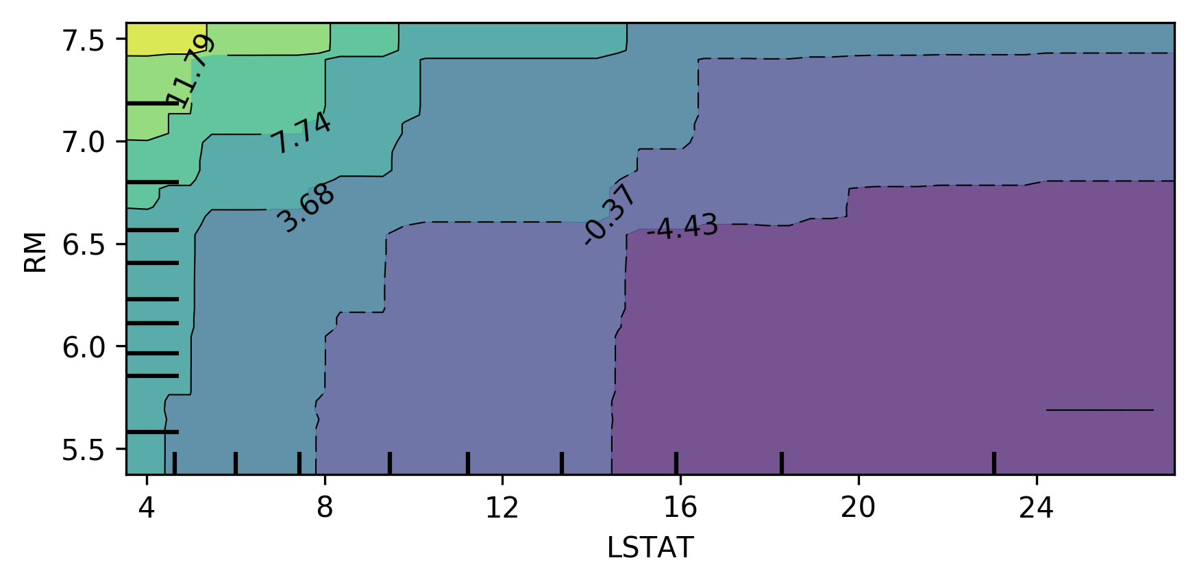
Bivariate Partial Dependence Plots

plot_partial_dependence(
    gbrt, X_train, [np.argsort(gbrt.feature_importances_)[-2:]],
    feature_names=boston.feature_names,
    n_jobs=3, grid_resolution=50)

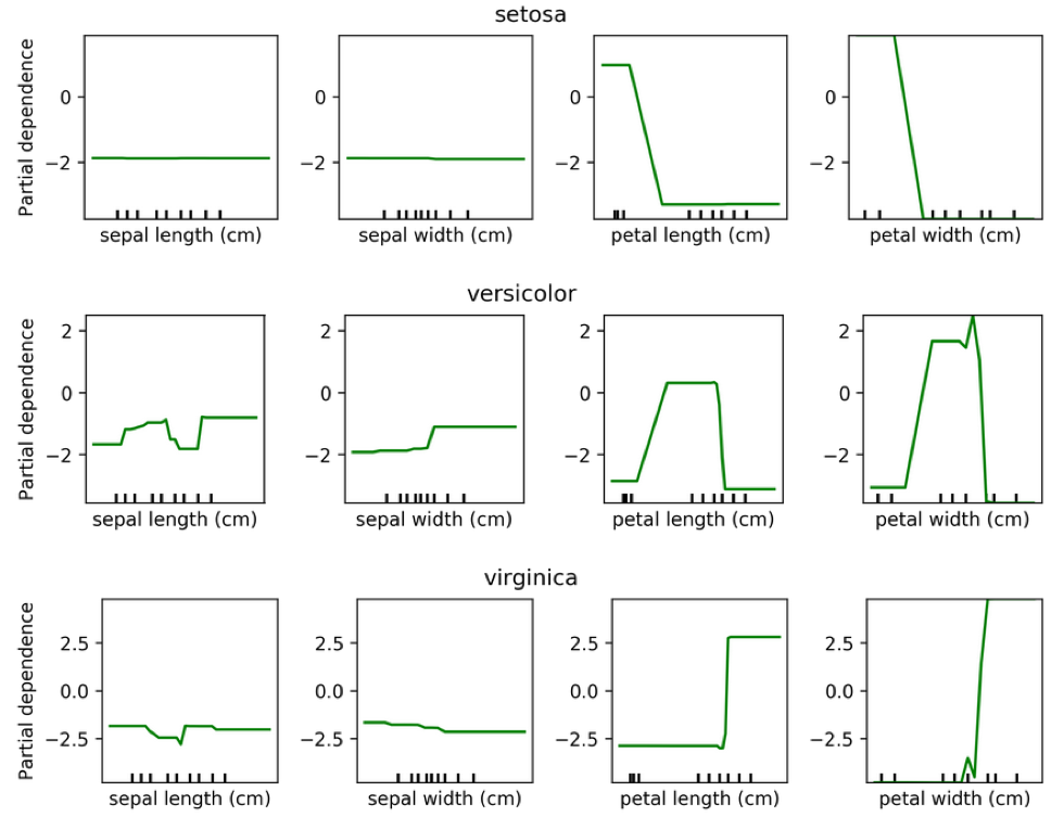
Partial Dependence for Classification

from sklearn.ensemble.partial_dependence import plot_partial_dependence
for i in range(3):
    fig, axs = \
        plot_partial_dependence(gbrt, X_train, range(4), n_cols=4,
                                feature_names=iris.feature_names,
                                grid_resolution=50, label=i)

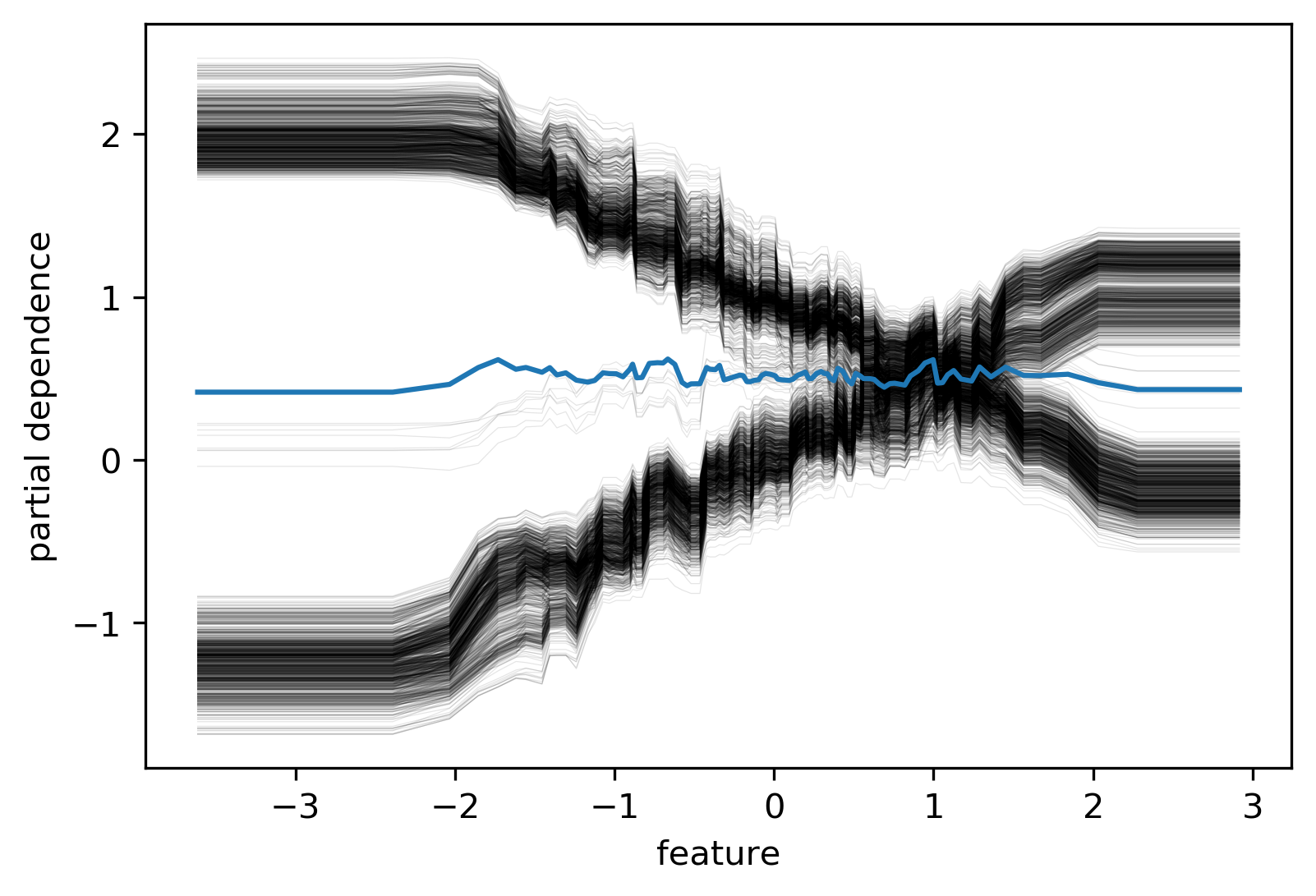
PDP Caveats

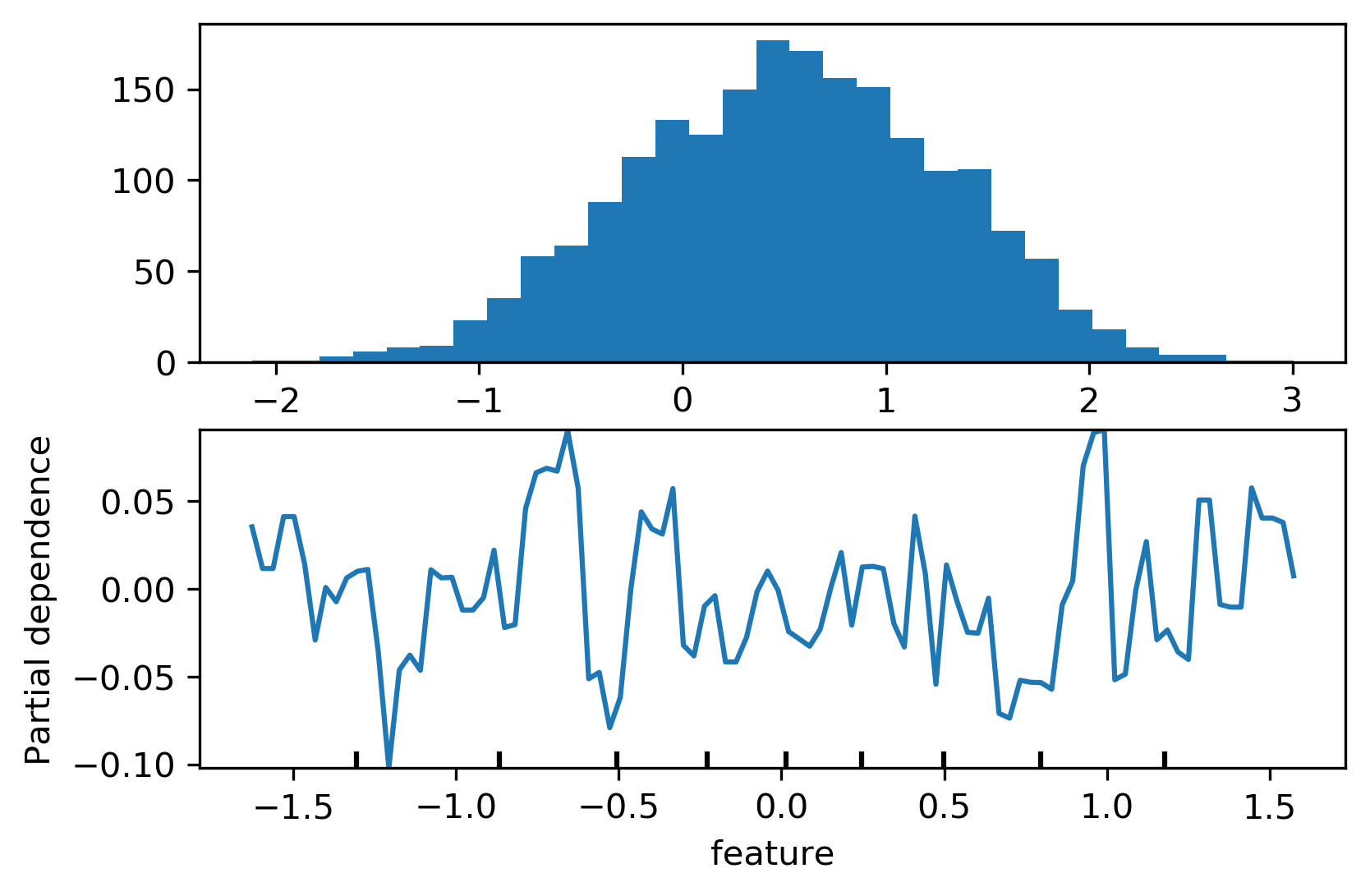
ICE (individual conditional expectation) plots

Like partial dependence plots, without averaging

See https://scikit-learn.org/stable/modules/partial_dependence.html

(Automatic) Feature Selection

Why Select Features?

Avoid overfitting (?)
Faster prediction and training
Less storage for model and dataset
More interpretable model

Types of Feature Selection

Unsupervised vs Supervised
Univariate vs Multivariate
Model based or not

Unsupervised Feature Selection

May discard important information
Variance-based: 0 variance or few unique values
Covariance-based: remove correlated features
PCA: remove linear subspaces

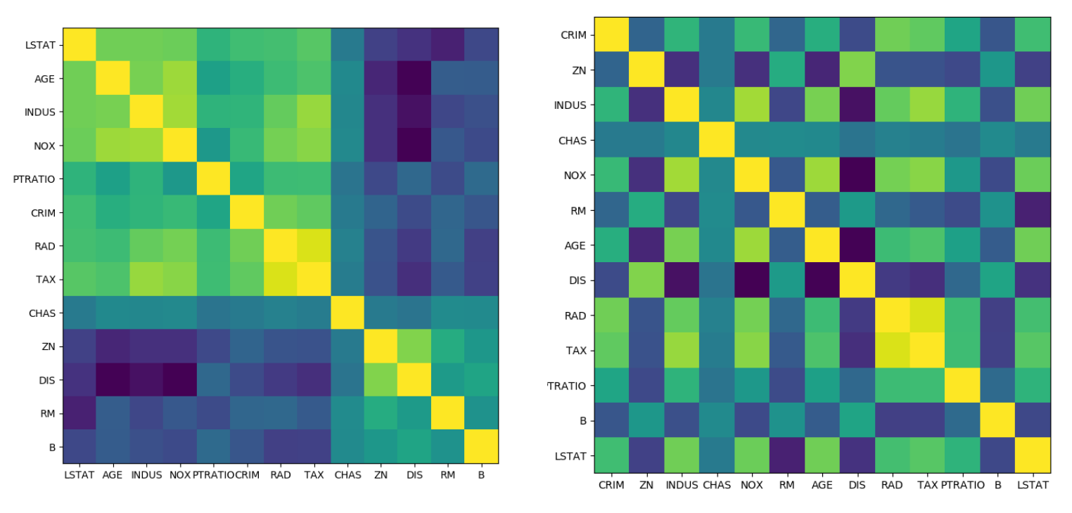
Covariance

from sklearn.preprocessing import scale
boston = load_boston()
X, y = boston.data, boston.target
X_train, X_test, y_train, y_test = \
    train_test_split(X, y, random_state=0)
X_train_scaled = scale(X_train)
cov = np.cov(X_train_scaled, rowvar=False)

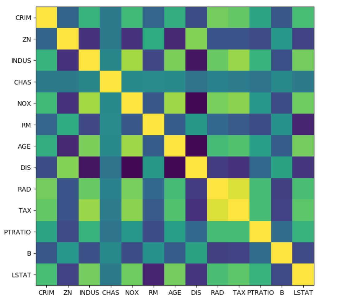
from scipy.cluster import hierarchy
order = np.array(hierarchy.dendrogram(
    hierarchy.ward(cov),no_plot=True)['ivl'], dtype="int")

Supervised Feature Selection

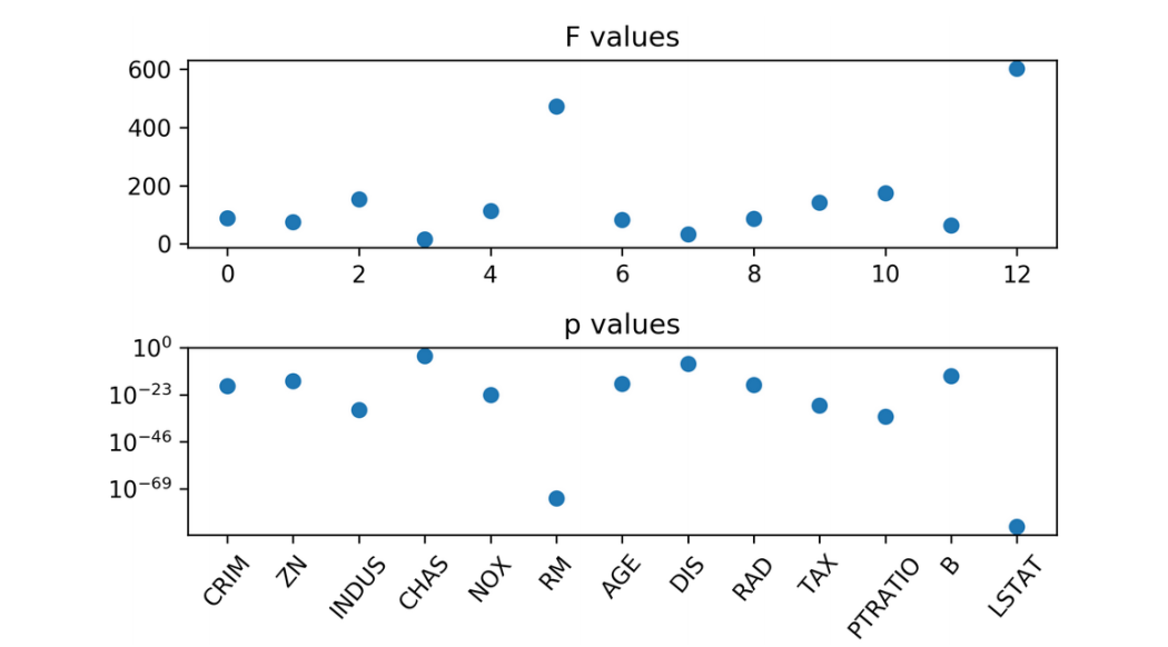
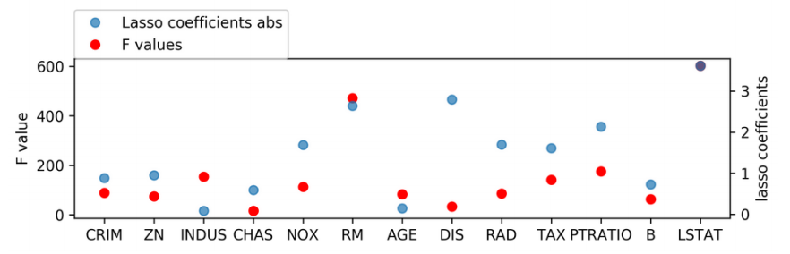
Univariate Statistics

Pick statistic, check p-values !
f_regression, f_classsif, chi2 in scikit-learn

from sklearn.feature_selection import f_regression
f_values, p_values = f_regression(X, y)

from sklearn.feature_selection import \
    SelectKBest, SelectPercentile, SelectFpr
from sklearn.linear_model import RidgeCV
select = SelectKBest(k=2, score_func=f_regression)
select.fit(X_train, y_train)
print(X_train.shape)
print(select.transform(X_train).shape)

(379, 13)
(379, 2)

all_features = make_pipeline(StandardScaler(), RidgeCV())
np.mean(cross_val_score(all_features, X_train, y_train, cv=10))

0.718

select_2 = make_pipeline(StandardScaler(),
                         SelectKBest(k=2,
                                     score_func=f_regression),
                         RidgeCV())
np.mean(cross_val_score(select_2, X_train, y_train, cv=10))

0.624

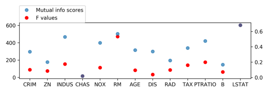
Mutual Information

from sklearn.feature_selection import mutual_info_regression
scores = mutual_info_regression(X_train, y_train,
                                discrete_features=[3])

Model-Based Feature Selection

Get best fit for a particular model
Ideally: exhaustive search over all possible combinations
Exhaustive is infeasible (and has multiple testing issues)
Use heuristics in practice.

Model based (single fit)

Build a model, select "features important to model"
Lasso, other linear models, tree-based Models
Multivariate - linear models assume linear relation

from sklearn.linear_model import LassoCV
X_train_scaled = scale(X_train)
lasso = LassoCV().fit(X_train_scaled, y_train)
print(lasso.coef_)

[-0.881 0.951 -0.082 0.59 -1.69 2.639 -0.146 -2.796 1.695 -1.614 -2.133 0.729 -3.615]

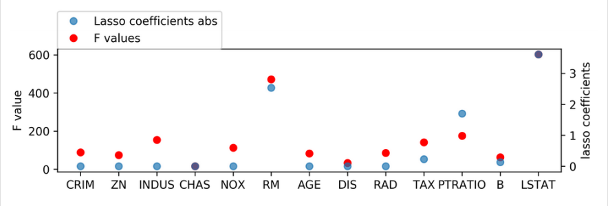
Changing Lasso alpha

from sklearn.linear_model import Lasso
X_train_scaled = scale(X_train)
lasso = Lasso().fit(X_train_scaled, y_train)
print(lasso.coef_)

[-0. 0. -0. 0. -0. 2.529 -0. -0. -0. -0.228 -1.701 0.132 -3.606]

`SelectFromModel`

from sklearn.feature_selection import SelectFromModel
select_lassocv = SelectFromModel(LassoCV(), threshold=1e-5)
select_lassocv.fit(X_train, y_train)
print(select_lassocv.transform(X_train).shape)

(379,11)

pipe_lassocv = make_pipeline(StandardScaler(),
                             select_lassocv, RidgeCV())
np.mean(cross_val_score(pipe_lassocv, X_train, y_train, cv=10))
np.mean(cross_val_score(all_features, X_train, y_train, cv=10))

0.717
0.718

# could grid-search alpha in lasso
select_lasso = SelectFromModel(Lasso())
pipe_lasso = make_pipeline(StandardScaler(), select_lasso, RidgeCV())
np.mean(cross_val_score(pipe_lasso, X_train, y_train, cv=10))

0.671

Iterative Model-Based Selection

Fit model, find least important feature, remove, iterate.
Or: Start with single feature, find most important feature, add, iterate.

Recursive Feature Elimination

Uses feature importances / coefficients, similar to “SelectFromModel”
Iteratively removes features (one by one or in groups)
Runtime: (n_features - n_feature_to_keep) / stepsize

from sklearn.linear_model import LinearRegression
from sklearn.feature_selection import RFE
# create ranking among all features by selecting only one
rfe = RFE(LinearRegression(), n_features_to_select=1)
rfe.fit(X_train_scaled, y_train)
rfe.ranking_

array([ 9, 8, 13, 11, 5, 2, 12, 4, 7, 6, 3, 10, 1])

RFECV

from sklearn.linear_model import LinearRegression
from sklearn.feature_selection import RFECV
rfe = RFECV(LinearRegression(), cv=10)
rfe.fit(X_train_scaled, y_train)
print(rfe.support_)
print(boston.feature_names[rfe.support_])

[ True  True False  True  True  True False  True  True  True  True  True True]
['CRIM' 'ZN' 'CHAS' 'NOX' 'RM' 'DIS' 'RAD' 'TAX' 'PTRATIO' 'B' 'LSTAT']

pipe_rfe_ridgecv = make_pipeline(StandardScaler(),
                                 RFECV(LinearRegression(),
                                       cv=10),
                                 RidgeCV())
np.mean(cross_val_score(pipe_rfe_ridgecv, X_train, y_train, cv=10))

0.710


pipe_rfe_ridgecv = make_pipeline(StandardScaler(),
                                 RFECV(LinearRegression(),
                                       cv=10),
                                 RidgeCV())
np.mean(cross_val_score(pipe_rfe_ridgecv, X_train, y_train, cv=10))

0.710

from sklearn.preprocessing import PolynomialFeatures
pipe_rfe_ridgecv = make_pipeline(StandardScaler(),
                                 PolynomialFeatures(),
                                 RFECV(LinearRegression(),
                                       cv=10),
                                 RidgeCV())
np.mean(cross_val_score(pipe_rfe_ridgecv, X_train, y_train, cv=10))

0.820

Wrapper methods

Can be applied for ANY model!
Shrink / grow feature set by greedy search
Called Forward or Backward selection
Run CV / train-val split per feature
Complexity: n_features * (n_features + 1) / 2
Implemented in mlxtend

`SequentialFeatureSelector`

from mlxtend.feature_selection import \
    SequentialFeatureSelector
sfs = SequentialFeatureSelector(LinearRegression(),
                                forward=False, k_features=7)
sfs.fit(X_train_scaled, y_train)

Features: 7/7

print(sfs.k_feature_idx_)
print(boston.feature_names[np.array(sfs.k_feature_idx_)])

(1, 4, 5, 7, 9, 10, 12)
['ZN' 'NOX' 'RM' 'DIS' 'TAX' 'PTRATIO' 'LSTAT']

sfs.k_score_

0.725