Ensembles

10/21/2022

Robert Utterback (based on slides by Andreas Muller)

\( \renewcommand{\vec}[1]{\boldsymbol{#1}} \newcommand{\E}{\mathop{\boldsymbol{E}}} \newcommand{\var}{\boldsymbol{Var}} \newcommand{\norm}[1]{\lvert\lvert#1\rvert\rvert} \newcommand{\abs}[1]{\lvert#1\rvert} \newcommand{\ltwo}[1]{\norm{#1}_2} \newcommand{\lone}[1]{\norm{#1}_1} \newcommand{\sgn}[1]{\text{sign}\left( #1 \right)} \newcommand{\e}{\mathrm{e}} \newcommand{\minw}{\min_{\vec{w} \in \mathbb{R}^p, b\in\mathbb{R}}} \newcommand{\summ}{\sum_{i=1}^m} \newcommand{\sumn}{\sum_{i=1}^n} \newcommand{\logloss}{\ln{(\exp{(-y^{(i)}(\vec{w}^T\vec{x}^{(i)}+b))} + 1)}} \newcommand{\ai}{\alpha^{(i)}} \newcommand{\w}{\vec{w}} \newcommand{\wt}{\vec{w}^T} \newcommand{\xi}{\vec{x}^{(i)}} \newcommand{\xit}{(\vec{x}^{(i)})^T} \newcommand{\xip}{\xit \vec{w}} \newcommand{\tip}{(\phi(\xi)^T \phi(\vec{x}))} \)

Ensemble Models

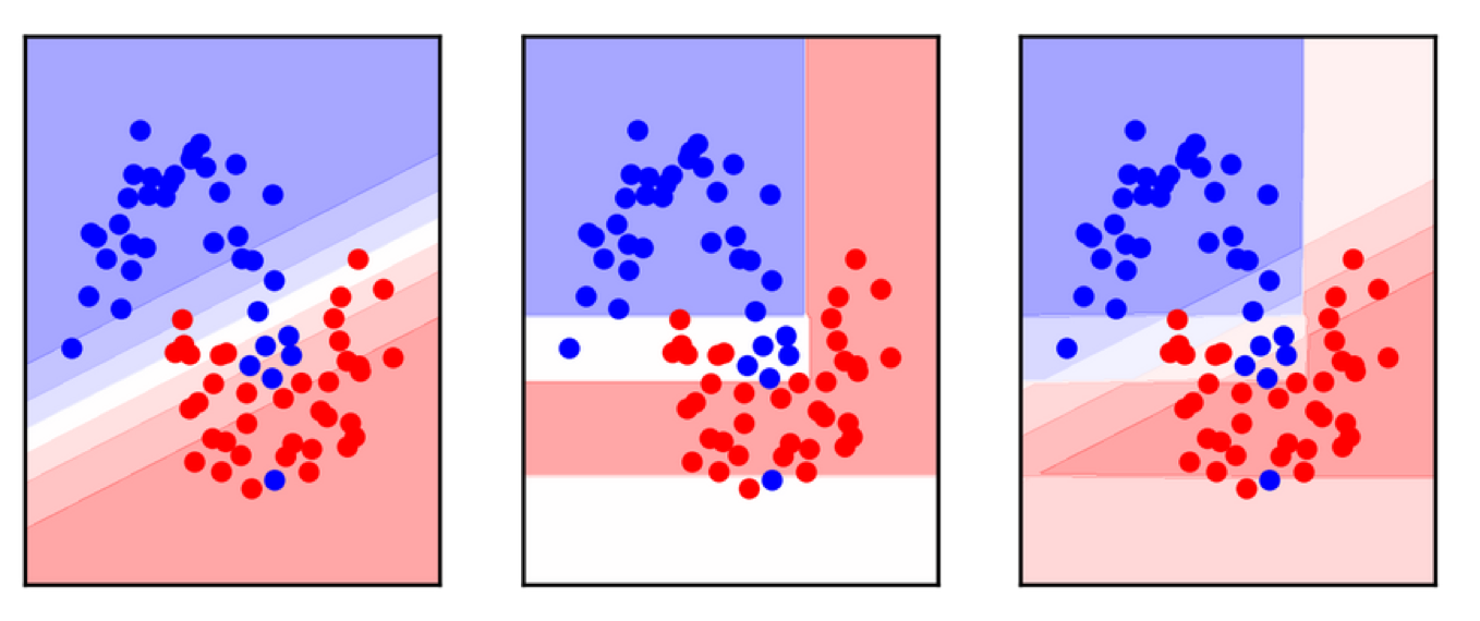
Poor man's ensembles

Build different models
Average the result
Owen Zhang (long time kaggle 1st): build XGBoosting models with different random seeds.
More models are better – if they are not correlated.
Also works with neural networks
You can average any models as long as they provide calibrated ("good") probabilities.
Scikit-learn: VotingClassifier hard and soft voting

VotingClassifier

voting = VotingClassifier(
    [('logreg', LogisticRegression(C=100)),
     ('tree', DecisionTreeClassifier(max_depth=3, random_state=0))],
    voting='soft')
voting.fit(X_train, y_train)
lr, tree = voting.estimators_
voting.score(X_test, y_test), lr.score(X_test, y_test), \
    tree.score(X_test, y_test)

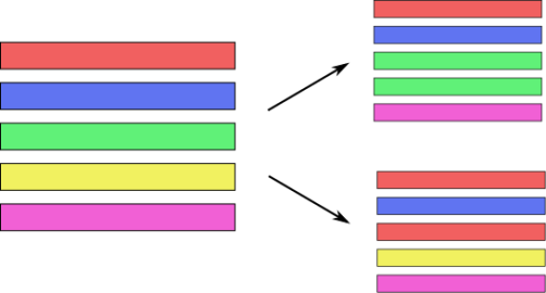
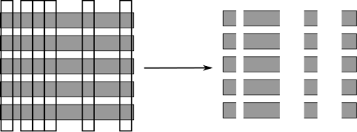
Bagging (Bootstrap Aggregation)

Generic way to build “slightly different” models
BaggingClassifier, BaggingRegressor

Bias and Variance

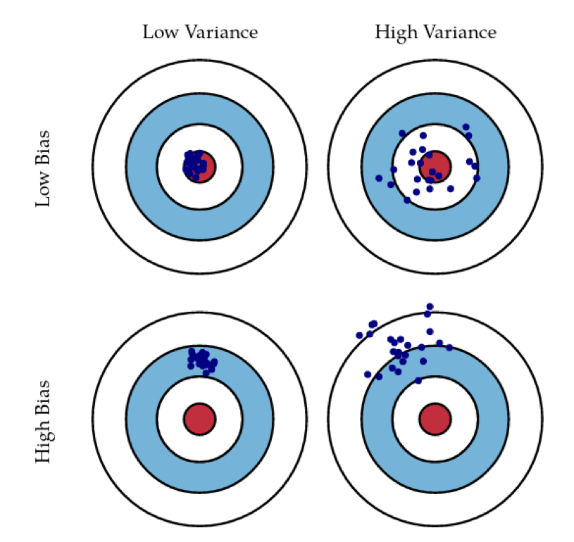
http://scott.fortmann-roe.com/docs/BiasVariance.html

Bias and Variance in Ensembles

Breiman showed that generalization depends on strength of the individual classifiers and (inversely) on their correlation
Uncorrelating them might help, even at the expense of strength

Random Forests

Forests

Build different trees
Average their results (or vote)

Random Forests

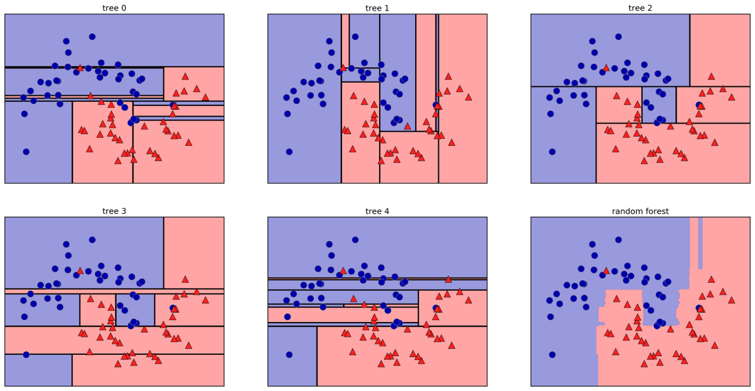
Tree Randomization

For each tree:
- Pick bootstrap sample of data
For each split:
- Pick random sample of features
More trees are always better

Tuning Random Forests

Main hyperparameter: max_features
- around sqrt(n_features) for classification
- Around n_features for regression
n_estimators > 100
Prepruning might help, definitely helps with model size!
max_depth, max_leaf_nodes, min_samples_split again

Extremely Randomized Trees

More randomness!
Randomly draw threshold for each feature
Doesn’t use bootstrap
Faster because no sorting / searching
Can have smoother boundaries

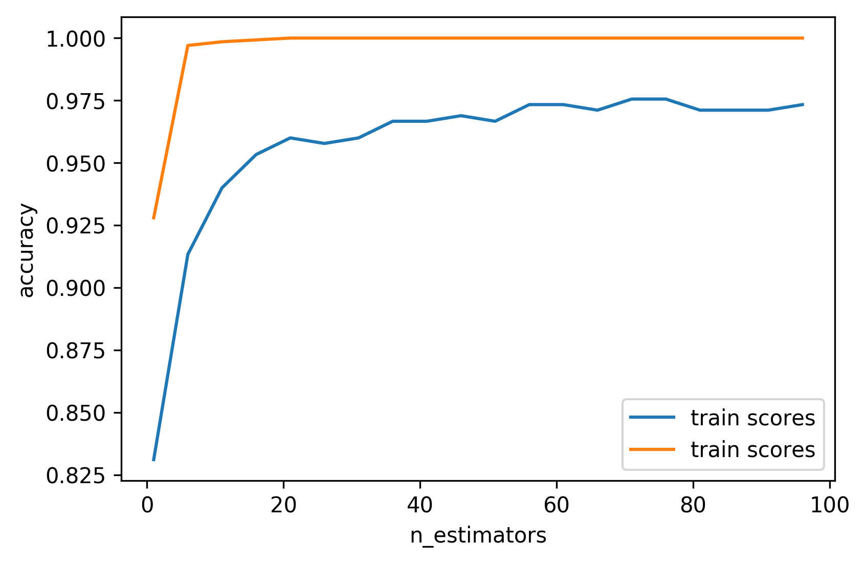
Warm-Starts

train_scores = []
test_scores = []

rf = RandomForestClassifier(warm_start=True)
estimator_range = range(1, 100, 5)
for n_estimators in estimator_range:
    rf.n_estimators = n_estimators
    rf.fit(X_train, y_train)
    train_scores.append(rf.score(X_train, y_train))
    test_scores.append(rf.score(X_test, y_test))

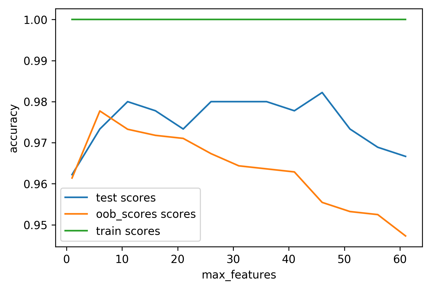
Out-of-bag estimates

Each tree only uses ~66% of data
Can evaluate it on the rest!
Make predictions for out-of-bag, average, score.
Each prediction is an average over different subset of trees

train_scores, test_scores, oob_scores = [], [], []

feature_range = range(1, 64, 5)
for max_features in feature_range:
    rf = RandomForestClassifier(max_features=max_features, oob_score=True,
                                n_estimators=200, random_state=0)
    rf.fit(X_train, y_train)
    train_scores.append(rf.score(X_train, y_train))
    test_scores.append(rf.score(X_test, y_test))
    oob_scores.append(rf.oob_score_)

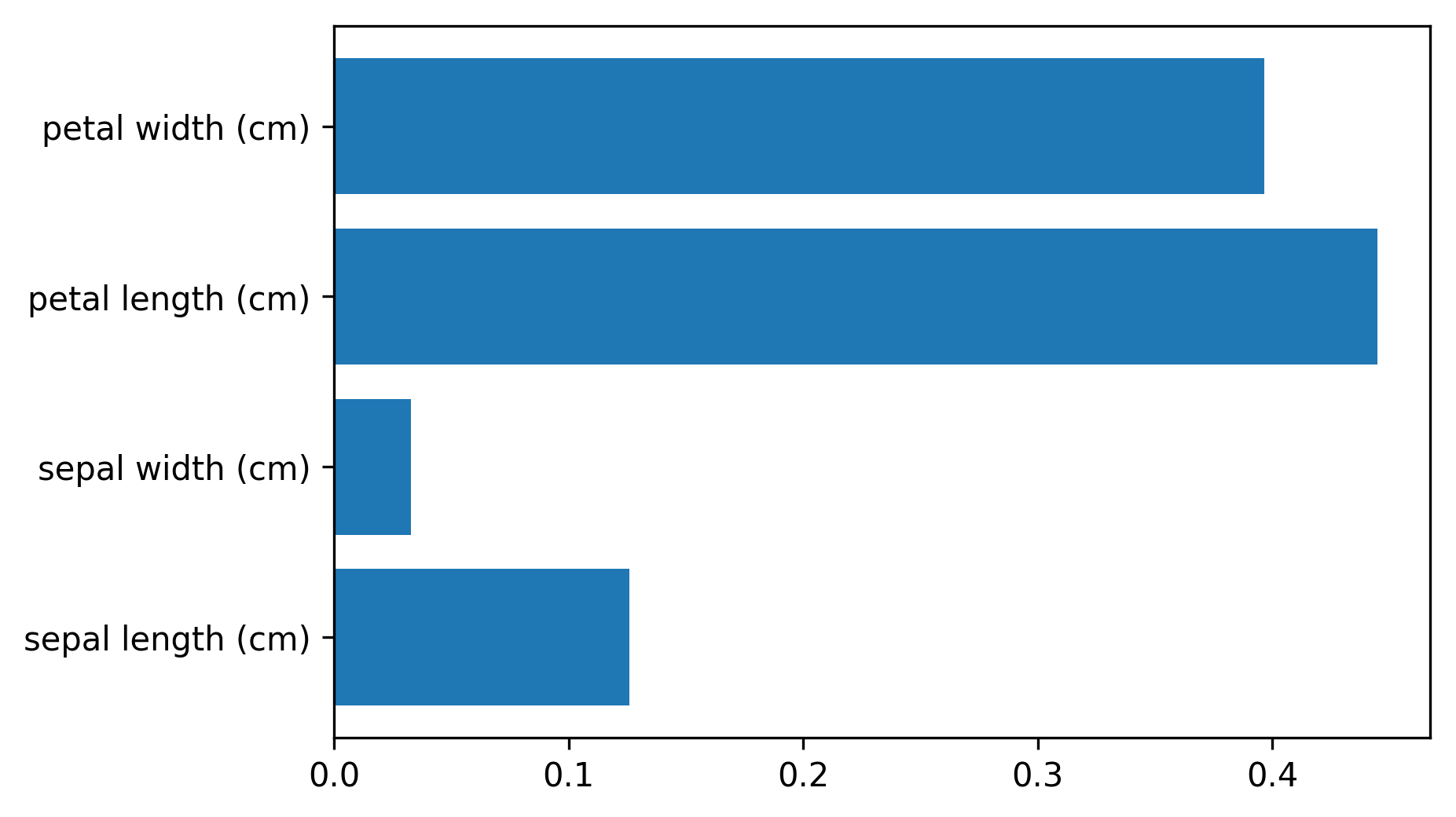
Variable Importance

X_train, X_test, y_train, y_test = \
    train_test_split(iris.data, iris.target,
                     stratify=iris.target, random_state=1)
rf = RandomForestClassifier(n_estimators=100).fit(X_train, y_train)
rf.feature_importances_
plt.barh(range(4), rf.feature_importances_)
plt.yticks(range(4), iris.feature_names);
# array([ 0.126,  0.033,  0.445,  0.396])

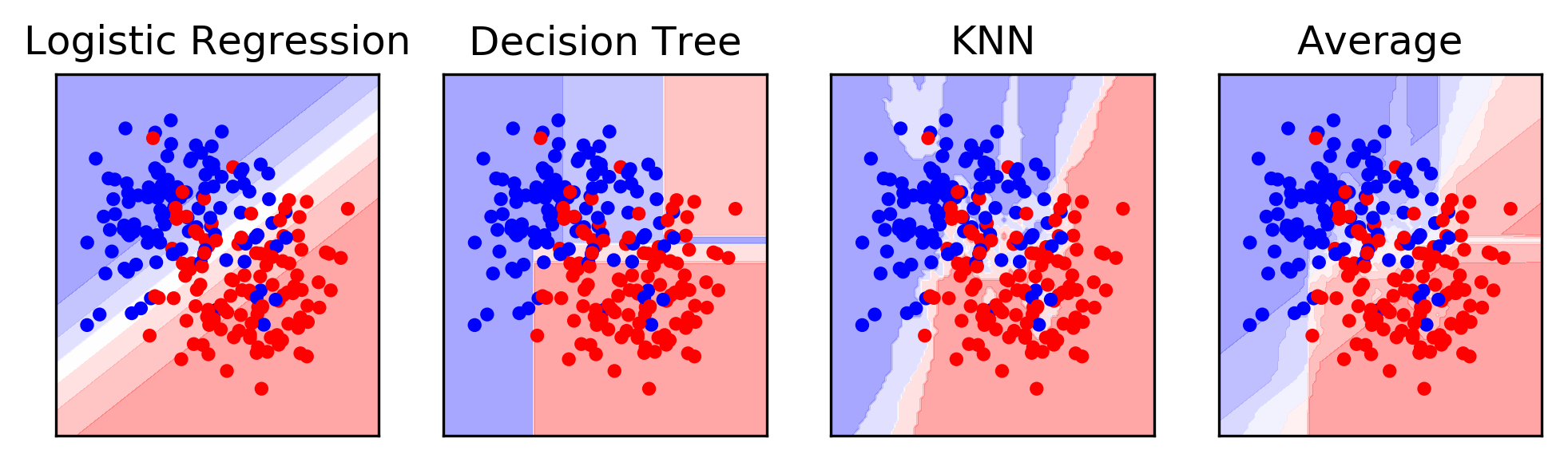
More ensembles: Stacking

Averaging

from sklearn.neighbors import KNeighborsClassifier

X, y = make_moons(noise=.4, random_state=16, n_samples=300)
X_train, X_test, y_train, y_test = \
    train_test_split(X, y, stratify=y, random_state=0)
voting = VotingClassifier(
   [('logreg', LogisticRegression(C=100)),
    ('tree', DecisionTreeClassifier(max_depth=3)),
    ('knn', KNeighborsClassifier(n_neighbors=3))],
    voting='soft')
voting.fit(X_train, y_train)
lr, tree, knn = voting.estimators_

Simplified Stacking

stacking = make_pipeline(voting, LogisticRegression(C=100))
stacking.fit(X_train, y_train)
stacking.named_steps.logisticregression.coef_

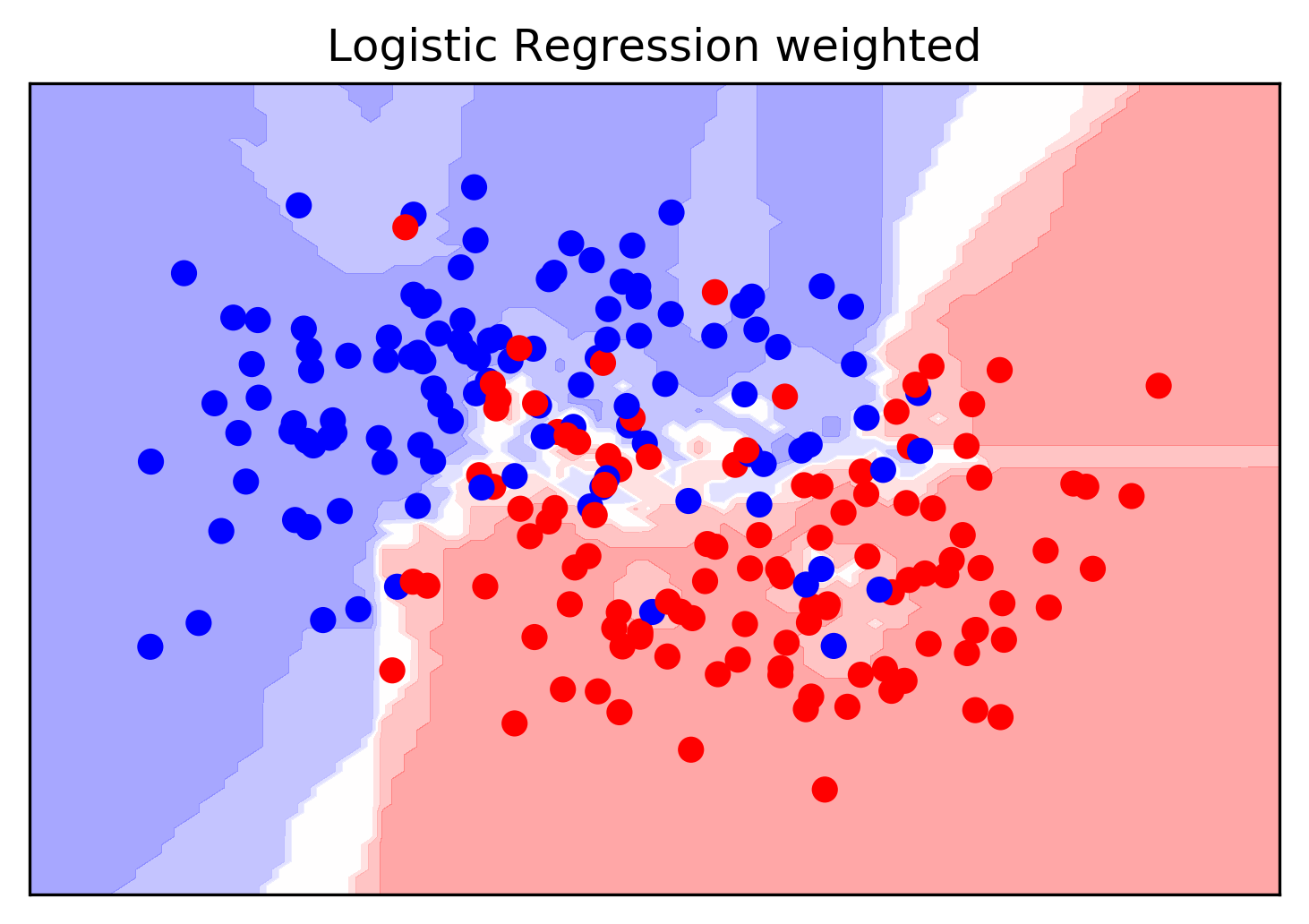
Problem: Overfitting!

Train first stage on training data
Second stage trains on probability estimates from training data
First stage overfitting -> most informative
Second stage will "trust" model that overfits the most

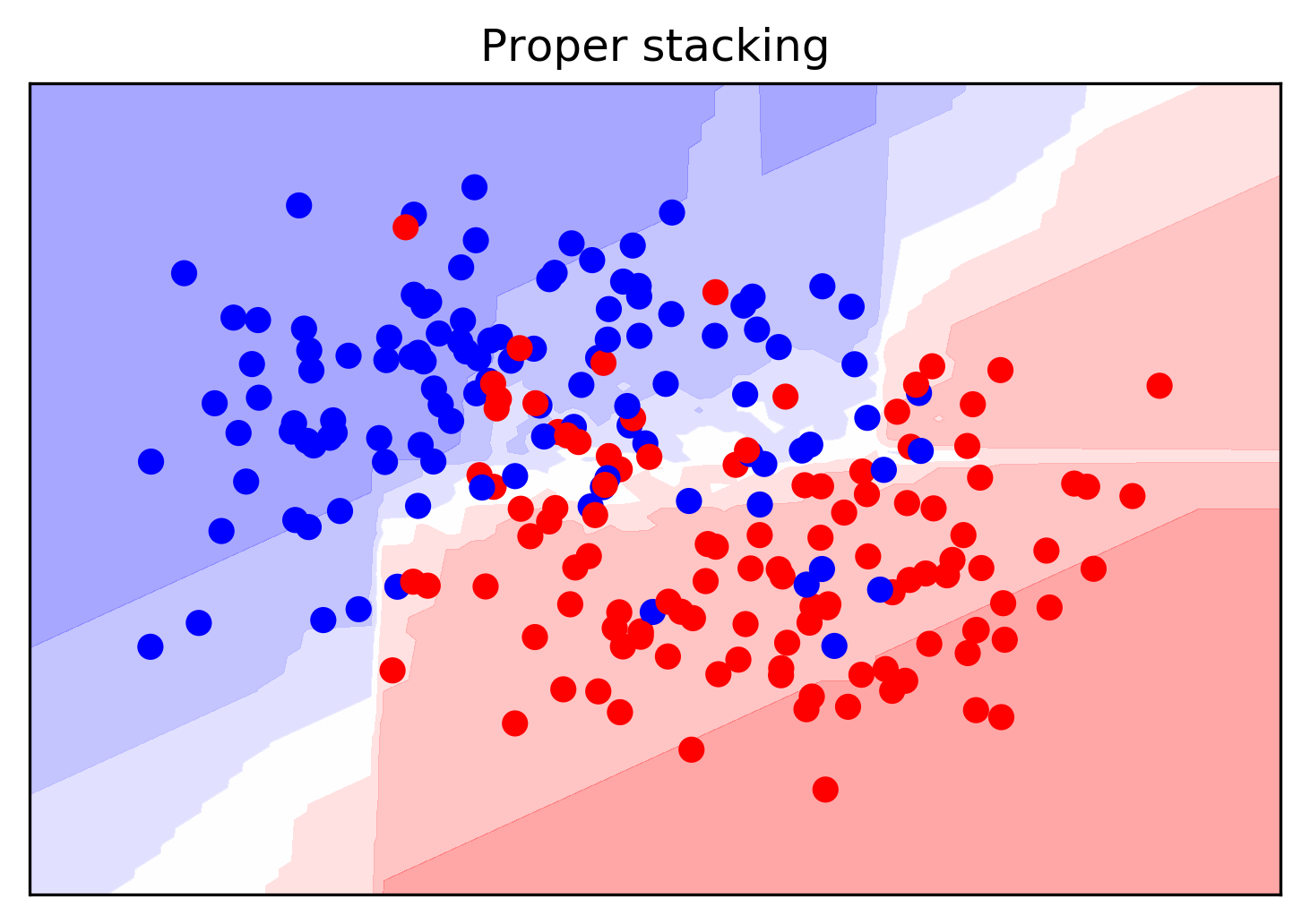
Stacking

Use validation set to produce prob. estimates
Train second step estimator on held-out estimates
No overfitting of second step!
For testing: as usual

Hold-out estimates of Probabilities

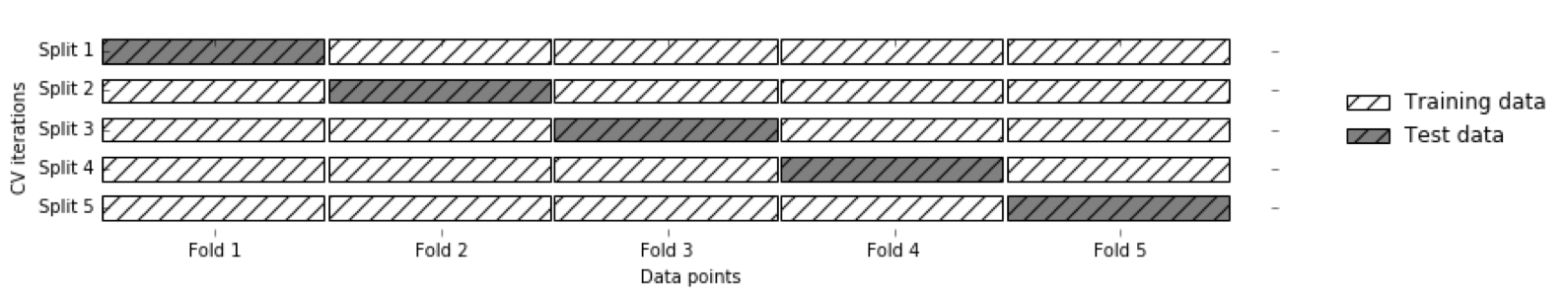
Split 1 produces probabilities for Fold 1, split2 for Fold 2 etc.
Get a probability estimate for each data point!
Unbiased estimates (like on the test set) for the whole training set!
Without it: The best estimator is the one that memorized the training set.

from sklearn.model_selection import cross_val_predict
# take only probabilities of positive classes for
# more interpretable coefficients
first_stage = make_pipeline(voting,
                            FunctionTransformer(lambda X: X[:, 1::2]))
transform_cv = cross_val_predict(first_stage, X_train,
                                 y_train, cv=10, method="transform")
second_stage = LogisticRegression(C=100).fit(transform_cv, y_train)
print(second_stage.coef_)
print(second_stage.score(transform_cv, y_train))
print(second_stage.score(first_stage.transform(X_test), y_test))

There are actually other ways to do this in sklearn. Here I'm specifying I want to use the "transform" method of the voting classifier. With voting='soft' and flatten_transform=True (the default), this gives back n_classifiers * n_classes columns, which is why I take every other column from it.

Use 10-fold CV to always just use transform on the held-out set (fold), i.e., just compute probabilities of the voting classifier on the hold-out set. So transform_cv is the same size as the training data set, so then we can use that to fit LogReg.

Q: Which model does it trust the most? A: the first, logreg. Now it doesn't trust kNN as much as before.

The goal of stacking is to blend different models in a smart way, making a more expressive model. The next thing seems similar but has a different goal.

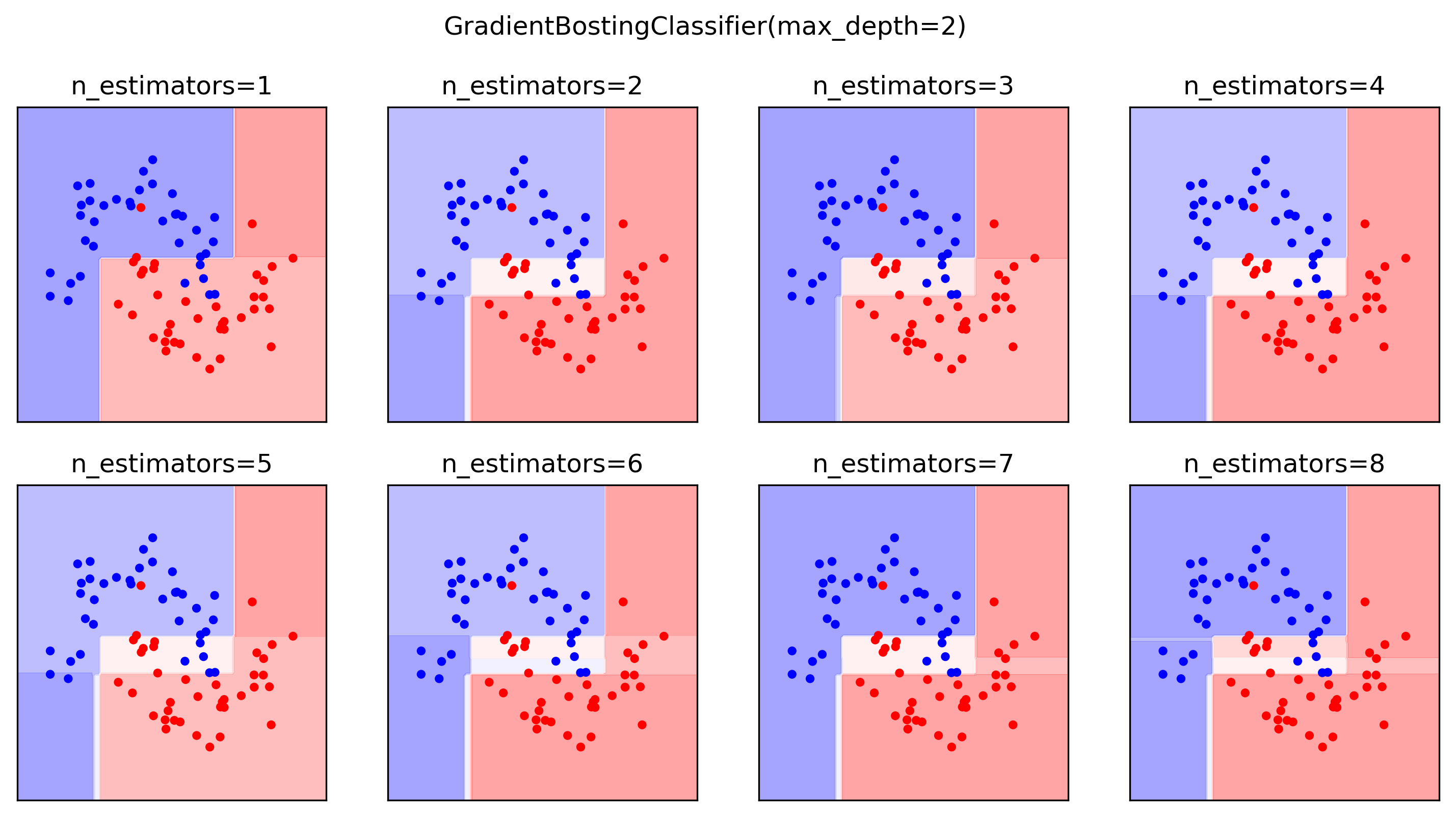
Boosting (in General)

One of the best off-the-shelf methods. Builds off of trees.

We'll continue on with the techniques of stacking and calibration.

Gradient boosting is one of the most successfull supervised machine learning methods in practice. It's often used in kaggle to win competition, it's used for credit scoring, it's one of the standard tools of the trade. It's one of the best of-the-shelf models.

A standard implementation that people use is XGBoost, but there's also an implementation in scikit-learn, and we'll talk about both of them. Last time we talked about Random forests, which builds many trees independently, each randomized in a different way, and then averages their predictions.

Gradient boosting on the other hand builds trees one by one in a sequential manner, with each tree requiring the results of previous trees. Often, Gradient boosting is done with very small trees, or even decision stumps, which is trees of depth one, so a single split.

"Meta-algorithm" (similar to bagging) to create strong learners from weak learners.
Tries to iteratively improve these simple (weak) models
AdaBoost, GentleBoost, …
Small Trees or stumps work best
Gradient Boosting often the best of the bunch, so we won't talk other types of boosting (or using other learners)
Many specialized algorithms (ranking etc)

This is an instance of a more general family of models, called boosting models, which all iteratively try to improve a model built up from weak learners. Gradient boosting is this particular technique where we are trying to fit the residuals, and it's been found to work very well in practice, in particular if you're using shallow trees as the weak learners. In principle, you could use any model as a weak learner, but trees just work really well.

Takeaway: boosting takes weak learners and makes them better; bagging reduces overfitting.

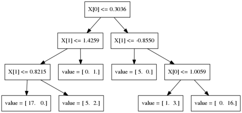
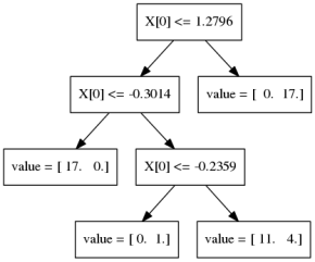
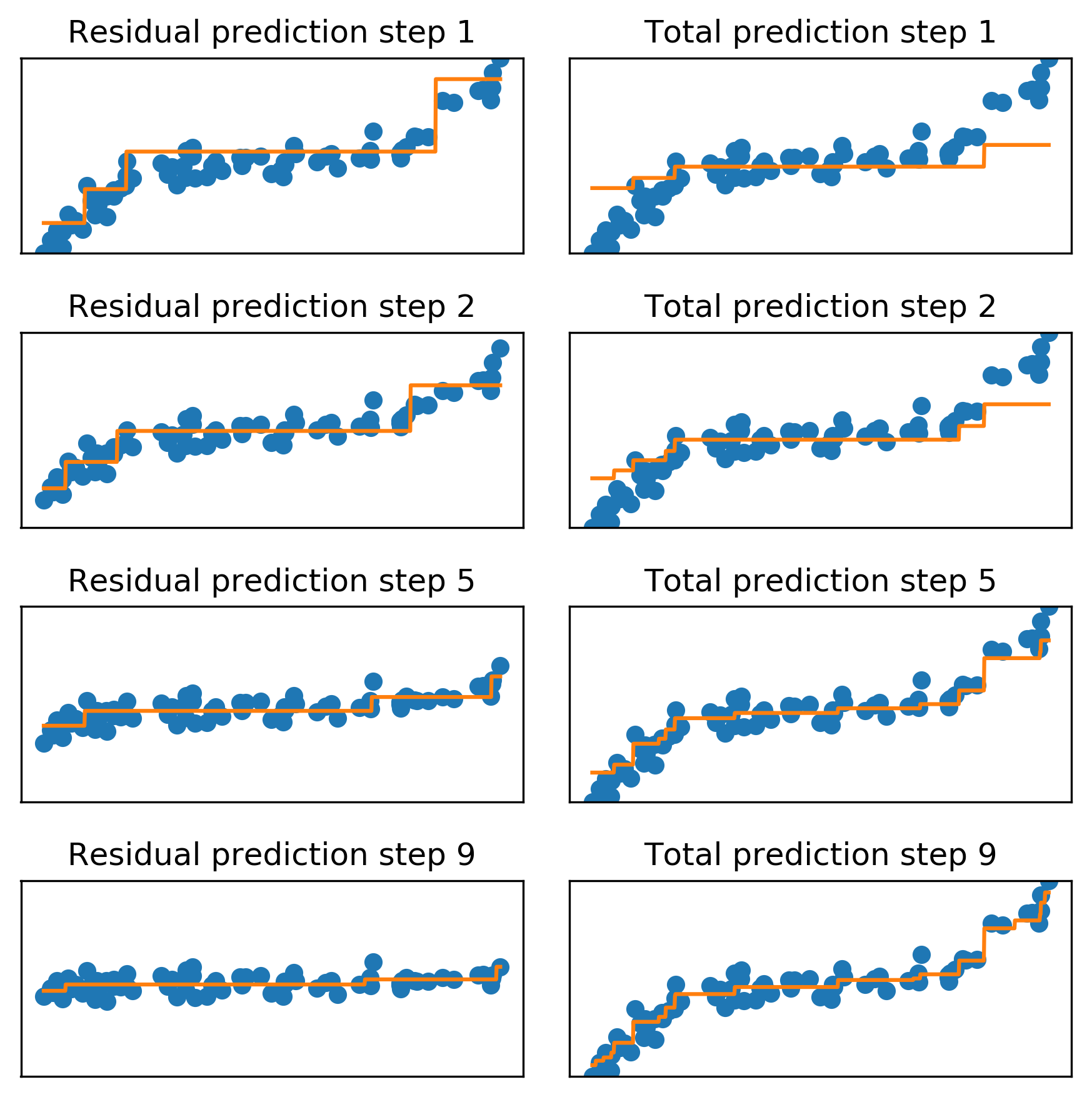
Gradient Boosting Algorithm

\[ f_{1}(x) \approx y \] \[ f_{2}(x) \approx y - f_{1}(x) \] \[ f_{3}(x) \approx y - f_{1}(x) - f_{2}(x)\]

\(y \approx\) + + + …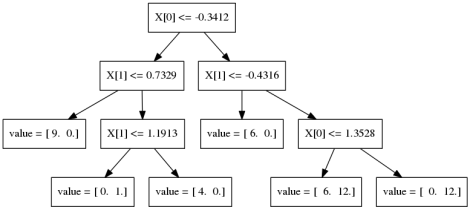

Let's look at the regression case first.
We start by building a single tree f1 to try to predict the output
1. But we strongly restrict f1 (shallow), so it will be rather bad at
predicting y.
Next, we'll look at the residual of this first model, so y - f1(x).
We now train a new model f2 to try and predict this residual, in other words to correct the mistakes made by f1. Again, this will be a very simple model, so it will still not be able to fix all errors.
Then, we look at the residual of both of the models together, so y - f1(x) - f2(x), so the mistakes that could not be fixed by f2, and we build f3 to fix that, and so on.
To make predictions you just add up all the predictions. Note you add, not average, like RF. Also in random forests each tree is independent.
This is natural for regression. For classification this is not as clear.
For binary classification you use log-loss, or rather you apply the logistic function to get a binary prediction, for multi-class you can use 1 vs rest.
So we're sequentially building up a model using what's called "weak learners", small trees, and create a more powerful composite model.

Learning Rate

\(f_{1}(x) \approx y\)

\(f_{2}(x) \approx y - \alpha f_{1}(x)\)

\(f_{3}(x) \approx y - \alpha f_{1}(x) - \alpha f_{2}(x)\)

\(y \approx \alpha\) + \(\alpha\) + \(\alpha\) + …

Learning rate \(\alpha, i.e. 0.1\)

GradientBoostingRegressor

GradientBoostingClassifier

Gradient Boosting Advantages

Slower to train than RF (serial), but much faster to predict
Small model size
Typically more accurate than Random Forests

Tuning Gradient Boosting

Pick n_estimators, tune learning rate
Can also tune max_features
Typically strong pruning via max_depth

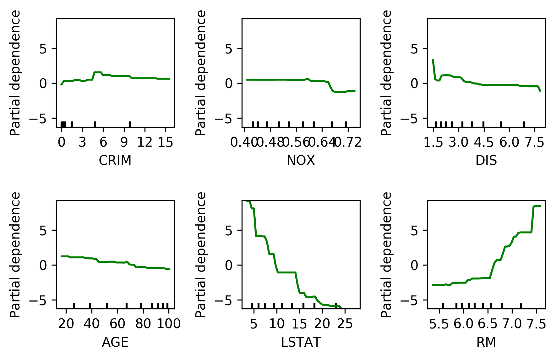
Analyzing Gradient Boosting

Partial Dependence Plots

Marginal dependence of prediction on one or two features

from sklearn.ensemble.partial_dependence import plot_partial_dependence
boston = load_boston()
X_train, X_test, y_train, y_test = \
    train_test_split(boston.data, boston.target,
                     random_state=0)

gbrt = GradientBoostingRegressor().fit(X_train, y_train)

fig, axs = \
    plot_partial_dependence(gbrt, X_train,
                            np.argsort(gbrt.feature_importances_)[-6:],
                            feature_names=boston.feature_names, n_jobs=3,
                            grid_resolution=50)

Partial Dependence Plots

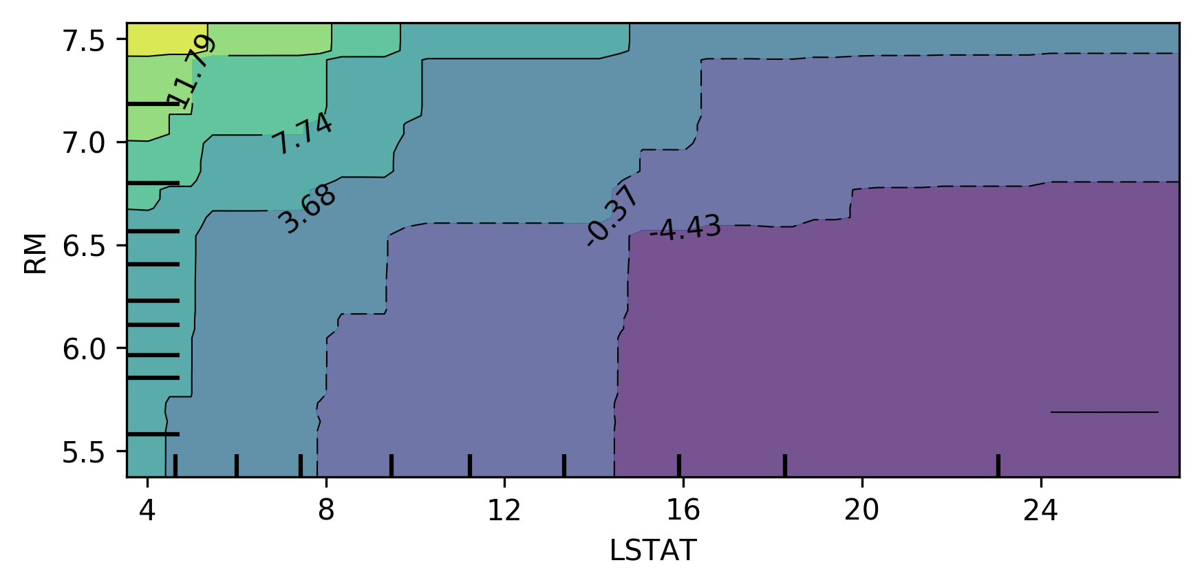
Bivariate Partial Dependence Plots

plot_partial_dependence(
    gbrt, X_train, [np.argsort(gbrt.feature_importances_)[-2:]],
    feature_names=boston.feature_names,
    n_jobs=3, grid_resolution=50)

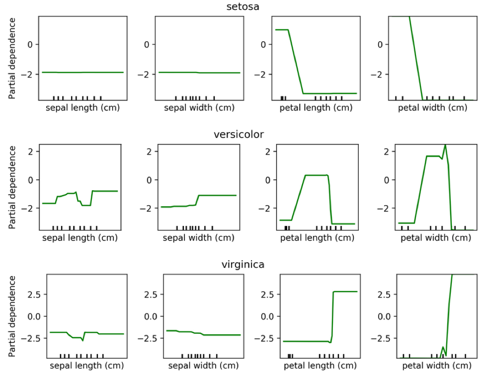
Partial Dependence for Classification

from sklearn.ensemble.partial_dependence import plot_partial_dependence
for i in range(3):
    fig, axs = \
        plot_partial_dependence(gbrt, X_train, range(4), n_cols=4,
                                feature_names=iris.feature_names,
                                grid_resolution=50, label=i)

Practical details

XGBoost

pip install xgboost

from xgboost import XGBClassifier
xgb = XGBClassifier()
xgb.fit(X_train, y_train)
xgb.score(X_test, y_test)

supports missing values
supports multi-core and GPU (sklearn does not)
Monotonicity constraints
Supports sparse data

Exact splits ~5x faster on single core
Approximate splits (bin the features, don't sort them), multi-core \(\to\) more speed!
Also check lightGBM (even faster?)

`LightGBM`

pip install lightgbm

from lightgbm.sklearn import LGBMClassifier
lgbm = LGBMClassifier()
lgbm.fit(X_train, y_train)
lgbm.score(X_test, y_test)

supports missing values
native support for categorical variables
multicore + GPU training
montonicity contraints
sparse data

`CatBoost`

pip install catboost

from catboost.sklearn import CatBoostClassifier
catb = CatBoostClassifier()
catb.fit(X_train, y_train)
catb.score(X_test, y_test)

optimized for categorical variables
uses one feature / threshold for all splits on a given level aka symmetric trees
Symmetric trees are "different" but can be much faster
supports missing value
GPU training
monotonicity constraints
uses bagged and smoothed version of target encoding for categorical variables
lots of tooling

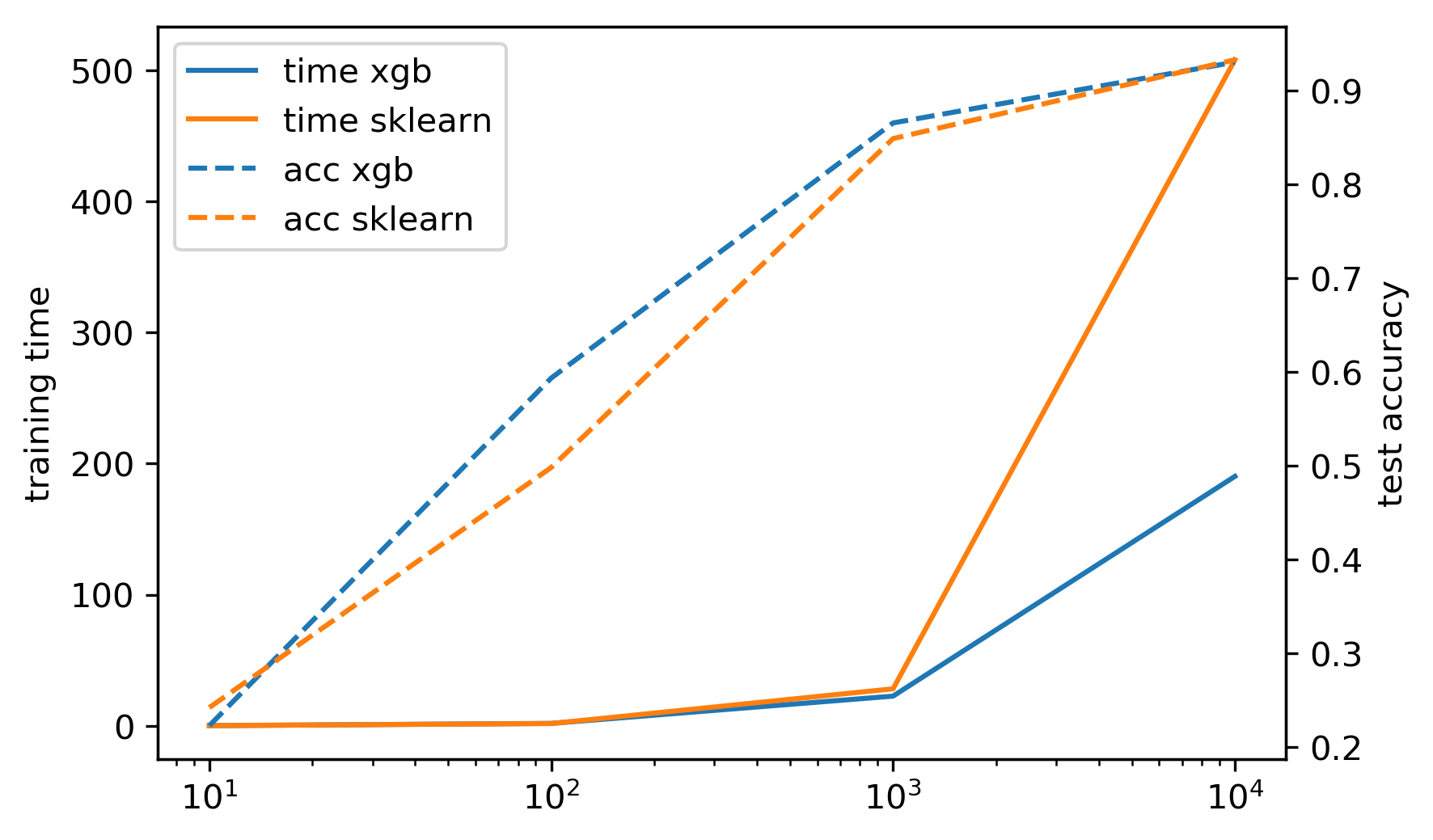
Newer `sklearn` Estimator

GradientBoostingClassifier

no feature 'binning'
single core
sparse data support

HistGradientBoostingClassifier

binning (makes training faster for \(m=10,000+\))
multicore
no sparse data support
missing value support (!)
monotonicity constraint support (!)
native categorical variables (must have numeric labels)

Early stopping

Adding trees can lead to overfitting
Stop adding trees when validation accuracy stops increasing
Optional in XGBoost and sklearn \(\ge\) 0.20

When to use tree-based models

Model non-linear relationships
Doesn’t care about scaling, no need for feature engineering
Single tree: very interpretable (if small)
Random forests: very robust, good benchmark
Gradient boosting often best performance with careful tuning

Dynamic Ensemble Selection

Motivation

letting all classifiers vote is dumb
Some classifiers good at some kinds of points, bad at others
(just like humans)
Idea: learn which classifiers are good for which "regions"

`DESlib` Quick Example

from deslib.des.knora_e import KNORAE
# 'pool' of 10 classifiers
pool_classifiers = RandomForestClassifier(n_estimators=10)
pool_classifiers.fit(X_train, y_train)
knorae = KNORAE(pool_classifiers) # init DES model
knorae.fit(X_dsel, y_dsel) # preprocess to find good 'regions'
knorae.predict(X_test) # predict

Ensembles

10/21/2022

Robert Utterback (based on slides by Andreas Muller)

Ensemble Models

Poor man's ensembles

VotingClassifier

Bagging (Bootstrap Aggregation)

Bias and Variance

Bias and Variance in Ensembles

Random Forests

Forests

Random Forests

Tree Randomization

Tuning Random Forests

Extremely Randomized Trees

Warm-Starts

Out-of-bag estimates

Variable Importance

More ensembles: Stacking

Averaging

Simplified Stacking

Problem: Overfitting!

Stacking

Hold-out estimates of Probabilities

Boosting (in General)

Gradient Boosting Algorithm

Learning Rate

GradientBoostingRegressor

GradientBoostingClassifier

Gradient Boosting Advantages

Tuning Gradient Boosting

Analyzing Gradient Boosting

Partial Dependence Plots

Partial Dependence Plots

Bivariate Partial Dependence Plots

Partial Dependence for Classification

Practical details

XGBoost

LightGBM

CatBoost

Newer sklearn Estimator

Early stopping

When to use tree-based models

Dynamic Ensemble Selection

Motivation

DESlib Quick Example

`LightGBM`

`CatBoost`

Newer `sklearn` Estimator

`DESlib` Quick Example