Decision Trees
10/17/2022
Robert Utterback (based on slides by Andreas Muller)
Decision Trees
Why Trees?
- Very powerful modeling method – non-linear!
- Don't care about scaling or distribution of data!
- Interpretable
- Basis of very powerful models!
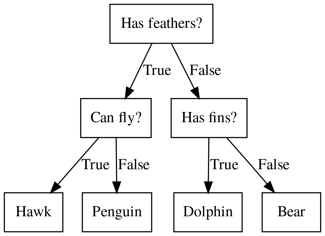
Decision Trees for Classification
Idea: series of binary questions
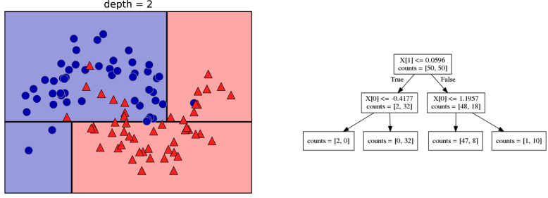
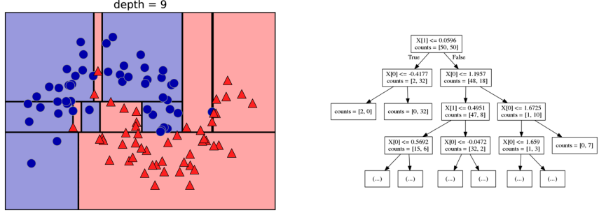
Building Trees (CART)
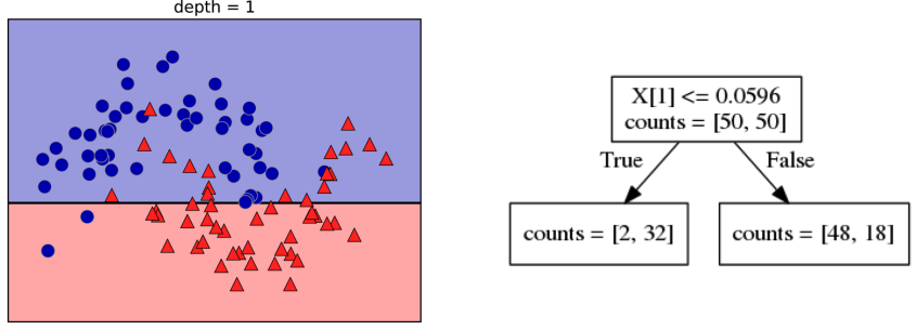
Continuous features:
- “questions” are thresholds on single features.
- Minimize impurity
Criteria (for classification)
- Gini Index: \(H_\text{gini}(X_m) = \sum_{k\in\mathcal{Y}} p_{mk} (1 - p_{mk})\)
- Cross-Entropy: \(H_\text{CE}(X_m) = -\sum_{k\in\mathcal{Y}} p_{mk} \log(p_{mk})\)
- \(x_m\) observations in node m
- \(\mathcal{Y}\) classes
- \(p_m\) distribution over classes in node m
Prediction

Regression trees
Regression Tree math
\[\text{Prediction: } \bar{y}_m = \frac{1}{N_m} \sum_{i \in N_m} y_i \]
\[ \text{Mean Squared Error: } H(X_m) = \frac{1}{N_m} \sum_{i \in N_m} (y_i - \bar{y}_m)^2 \]
\[ \text{Mean Absolute Error: } H(X_m) = \frac{1}{N_m} \sum_{i \in N_m} |y_i - \bar{y}_m| \]
Visualizing Trees
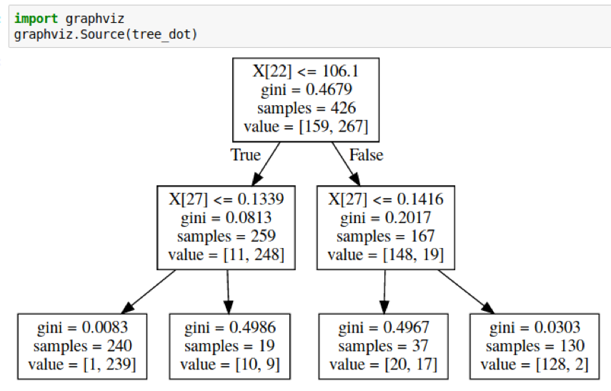
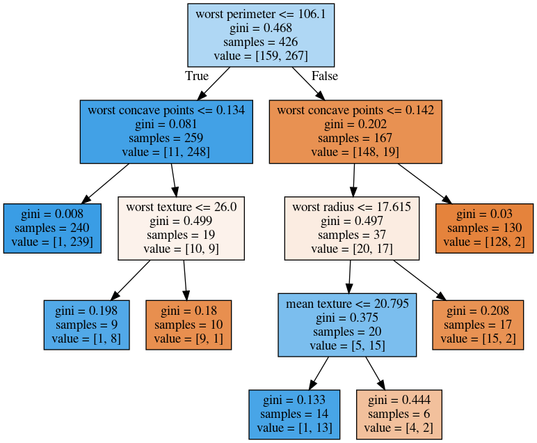
Visualizing trees with sklearn
from sklearn.datasets import load_breast_cancer
cancer = load_breast_cancer()
X_train, X_test, y_train, y_test = \
    train_test_split(cancer.data,cancer.target,
                     stratify=cancer.target,
                     random_state=0)
from sklearn.tree import DecisionTreeClassifier, \
    export_graphviz
tree = DecisionTreeClassifier(max_depth=2)
tree.fit(X_train, y_train)
# tree visualization (or sklearn.tree.plot_tree)
tree_dot = export_graphviz(tree, out_file=None,
                           feature_names=cancer.feature_names)
print(tree_dot)
Visualizing trees with sklearn
digraph Tree {
node [shape=box, fontname="helvetica"] ;
edge [fontname="helvetica"] ;
0 [label="worst perimeter <= 106.1\ngini = 0.468\nsamples = 426\nvalue = [159, 267]"] ;
1 [label="worst concave points <= 0.134\ngini = 0.081\nsamples = 259\nvalue = [11, 248]"] ;
0 -> 1 [labeldistance=2.5, labelangle=45, headlabel="True"] ;
2 [label="gini = 0.008\nsamples = 240\nvalue = [1, 239]"] ;
1 -> 2 ;
3 [label="gini = 0.499\nsamples = 19\nvalue = [10, 9]"] ;
1 -> 3 ;
4 [label="worst concave points <= 0.142\ngini = 0.202\nsamples = 167\nvalue = [148, 19]"] ;
0 -> 4 [labeldistance=2.5, labelangle=-45, headlabel="False"] ;
5 [label="gini = 0.497\nsamples = 37\nvalue = [20, 17]"] ;
4 -> 5 ;
6 [label="gini = 0.03\nsamples = 130\nvalue = [128, 2]"] ;
4 -> 6 ;
}
Showing dot files in Jupyter
Requires graphviz C library and Python library
!pip install graphviz
Producing Images from Command Line
dot -Tpng cancer_tree.dot -o cancer_tree.png
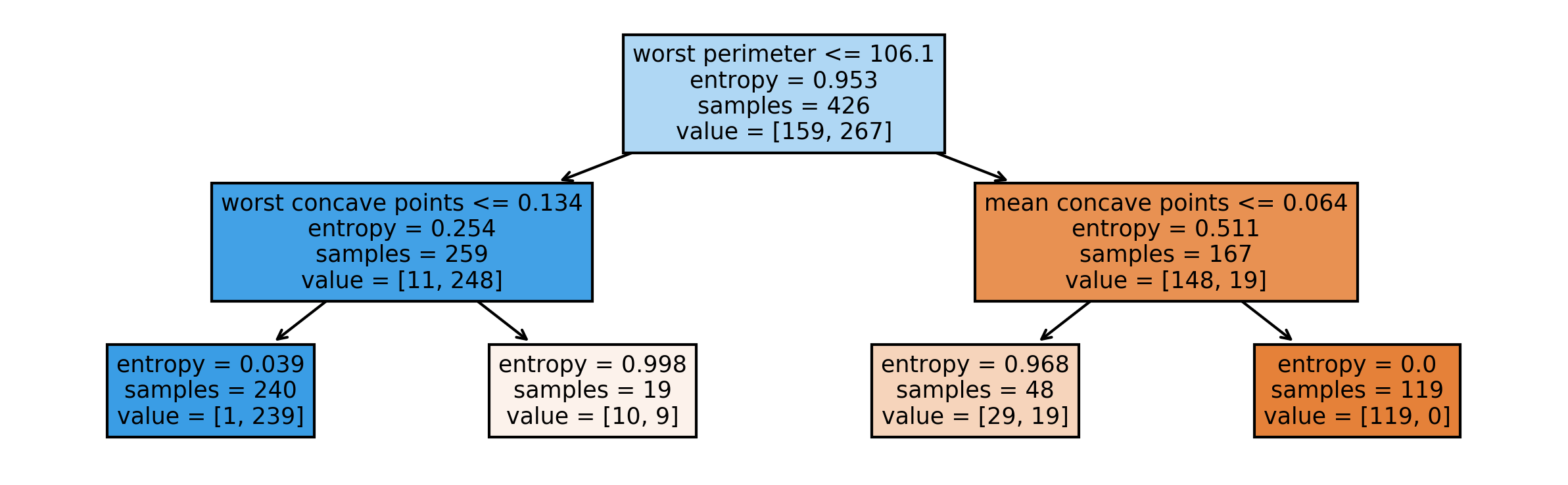
Visualizing Trees Directly with sklearn
  from sklearn.tree import plot_tree
  tree_dot = plot_tree(tree, feature_names=cancer.feature_names)
Parameter Tuning
Parameters
- Pre-pruning and post-pruning
- Limit tree size (pick one, maybe two):
max_depthmax_leaf_nodesmin_samples_splitmin_impurity_decrease
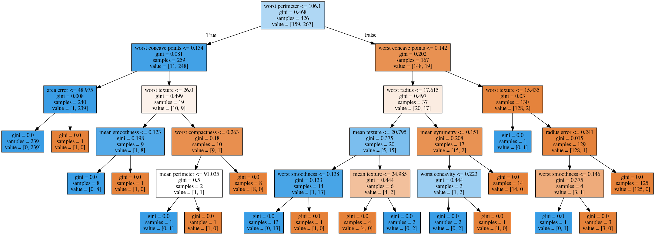
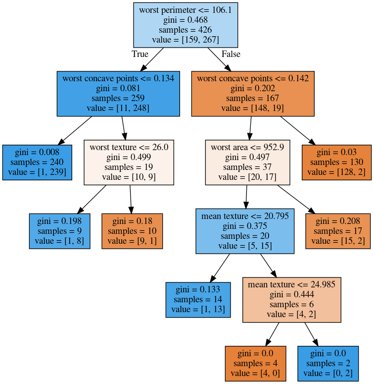
No pruning
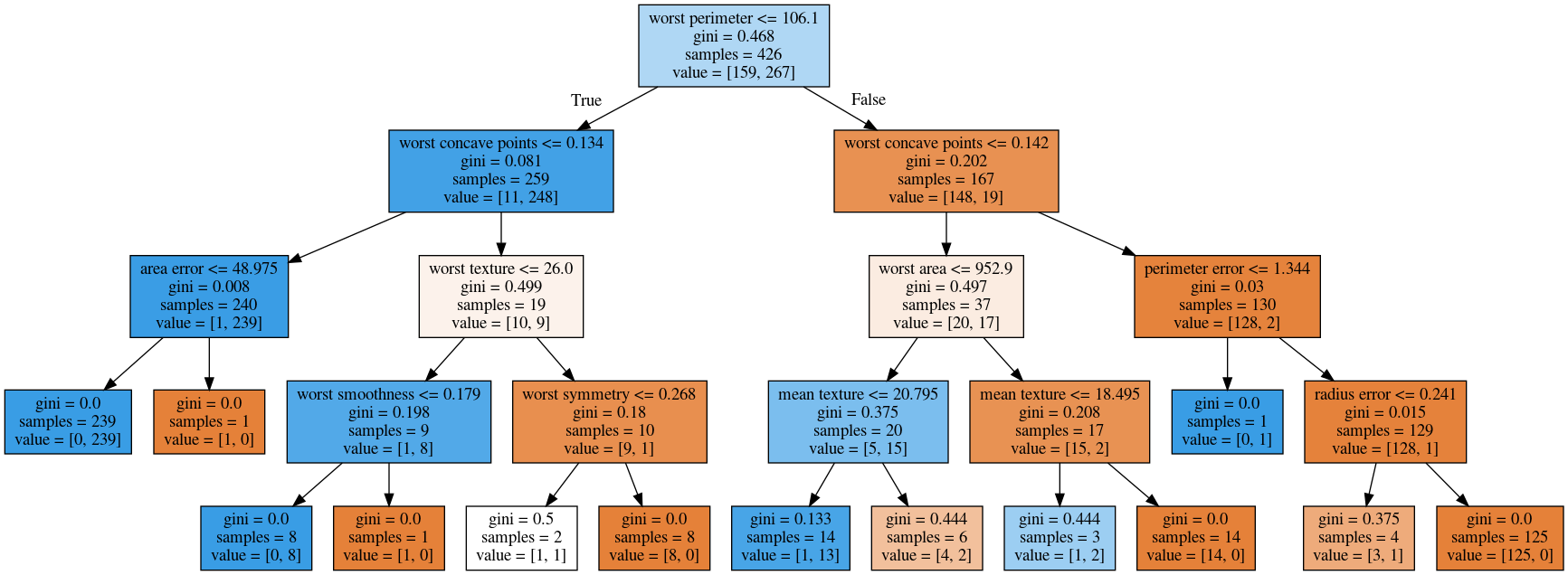
max_depth = 4
max_leaf_nodes = 8
min_samples_split = 50
from sklearn.model_selection import GridSearchCV
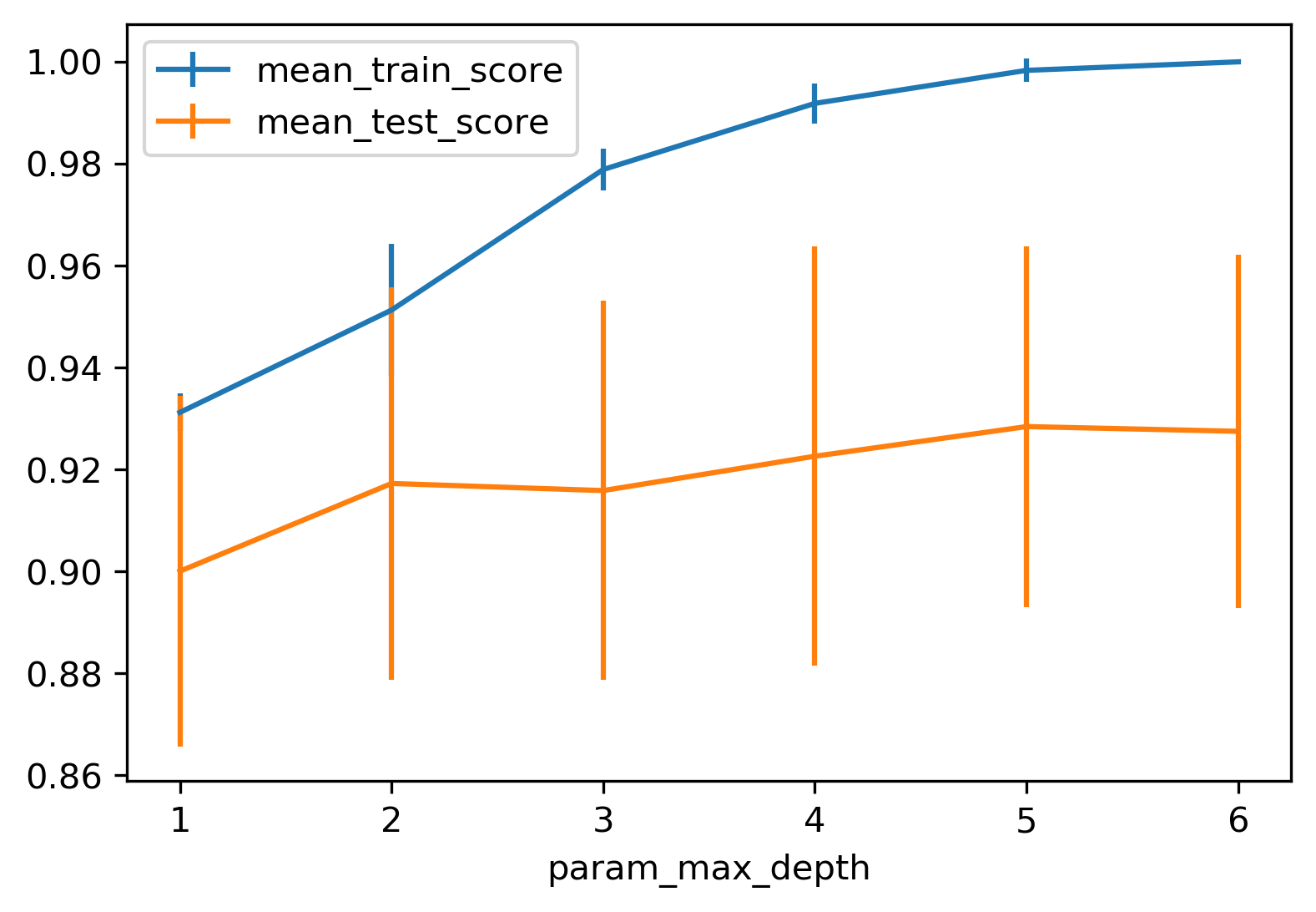
param_grid = {'max_depth':range(1, 7)}
grid = GridSearchCV(DecisionTreeClassifier(random_state=0),
param_grid=param_grid,
cv=10)
grid.fit(X_train, y_train)
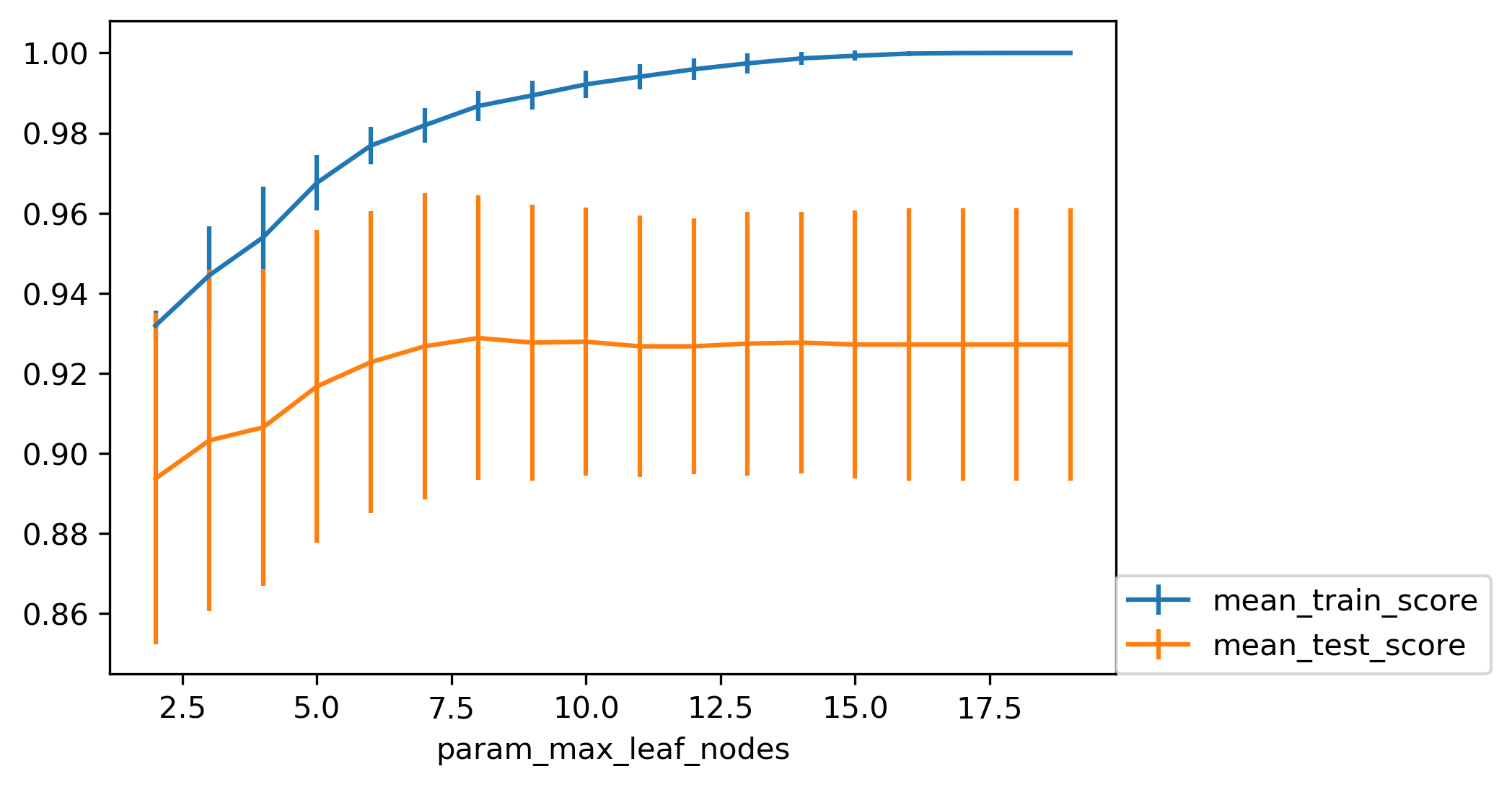
from sklearn.model_selection import GridSearchCV
param_grid = {'max_leaf_nodes':range(2, 20)}
grid = GridSearchCV(DecisionTreeClassifier(random_state=0),
                    param_grid=param_grid, cv=10)
grid.fit(X_train, y_train)
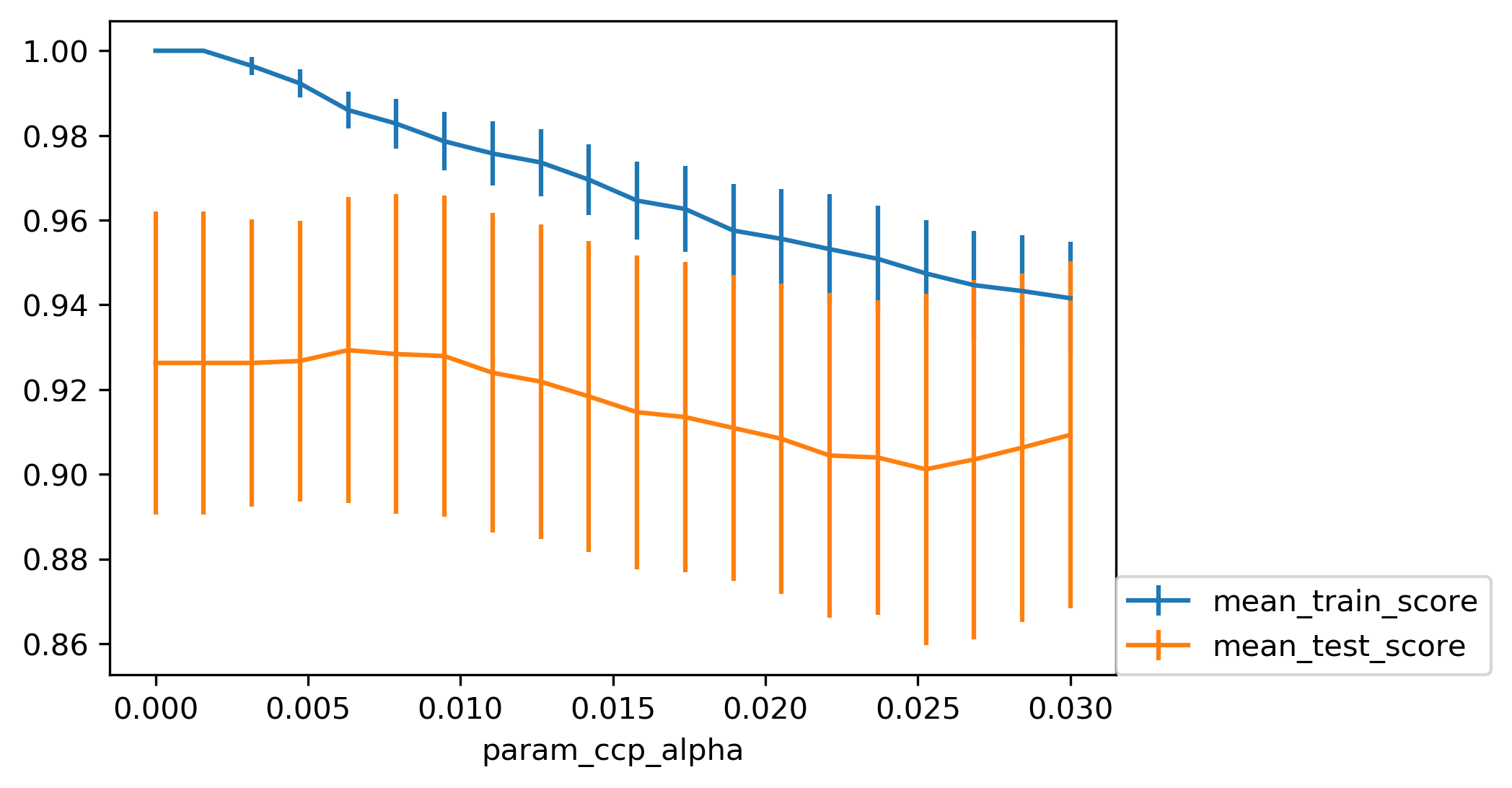
Cost Complexity (Post-) Pruning
\[ R_\alpha(T) = R(T) + \alpha |T| \]
- \(R(T)\) is total leaf impurity
- \(|T|\) is number of leaf nodes
- \(\alpha\) is hyperparameter
  param_grid = {'ccp_alpha': np.linspace(0.0, 0.03, 20)}
  grid = GridSearchCV(DecisionTreeClassifier(random_state=0),
		      param_grid=param_grid, cv=10)
  grid.fit(X_train, y_train)
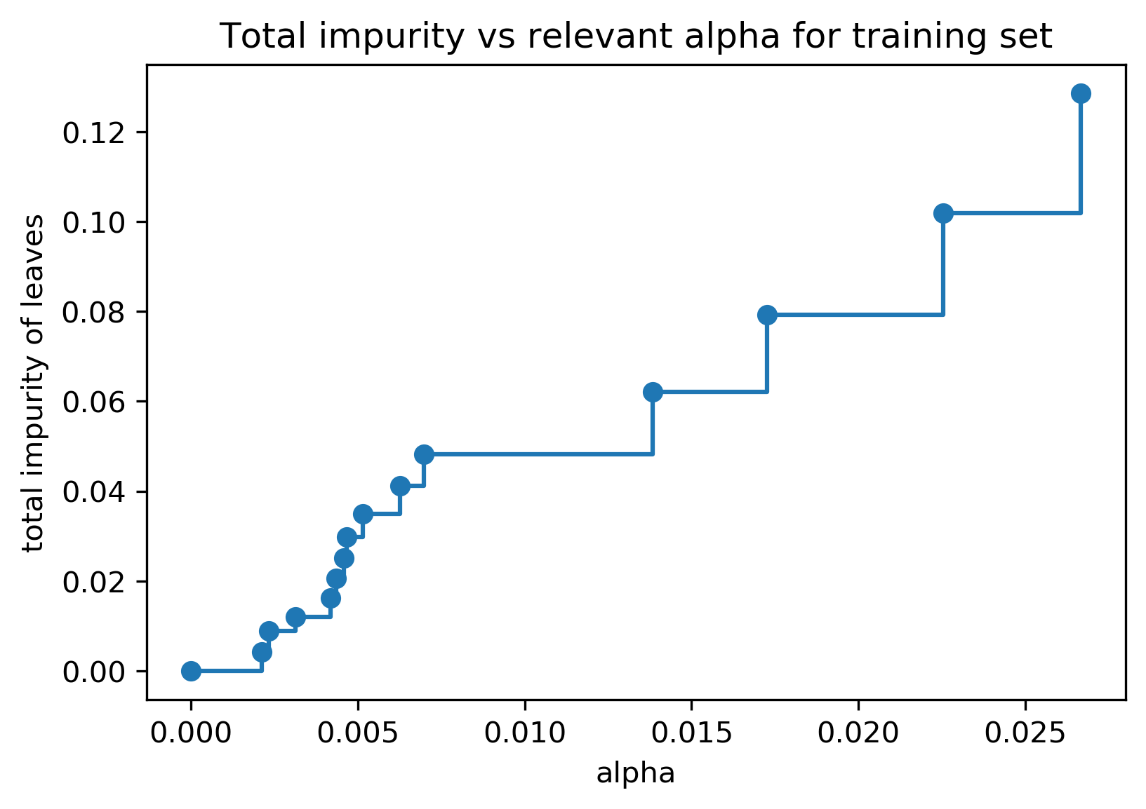
Efficient Pruning
  clf = DecisionTreeClassifier(random_state=0)
  path = clf.cost_complexity_pruning_path(X_train, y_train)
  ccp_alphas, impurities = path.ccp_alphas, path.impurities
Post-pruned vs. Pre-pruned
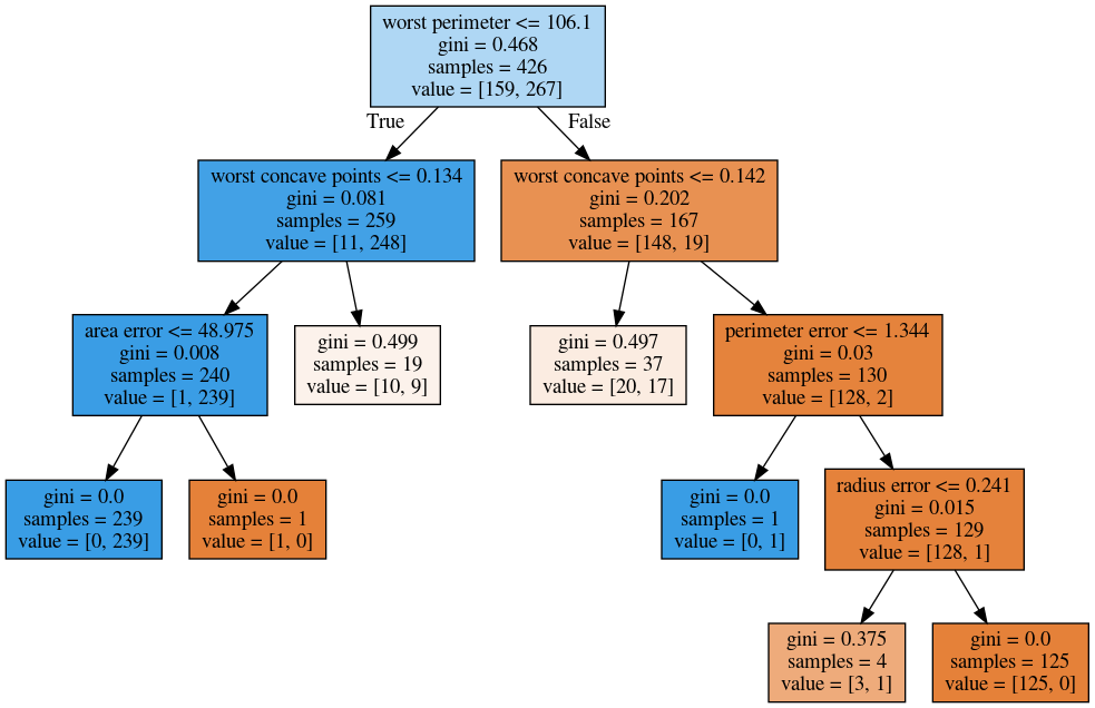
Cost-complexity pruning
Max leaf nodes search
Weaknesses
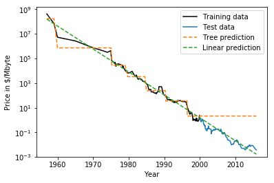
RAM Price over Time
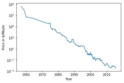
Extrapolation
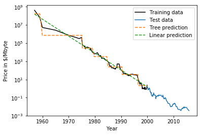
Extrapolation
Relation to Nearest Neighbors
- Predict average of neighbors – either by k, by epsilon ball or by leaf.
- Trees are much faster to predict.
- Neither can extrapolate
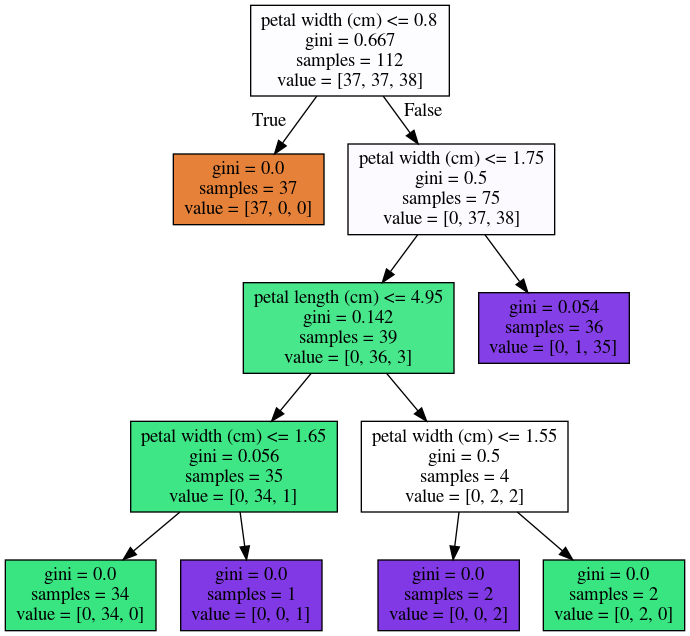
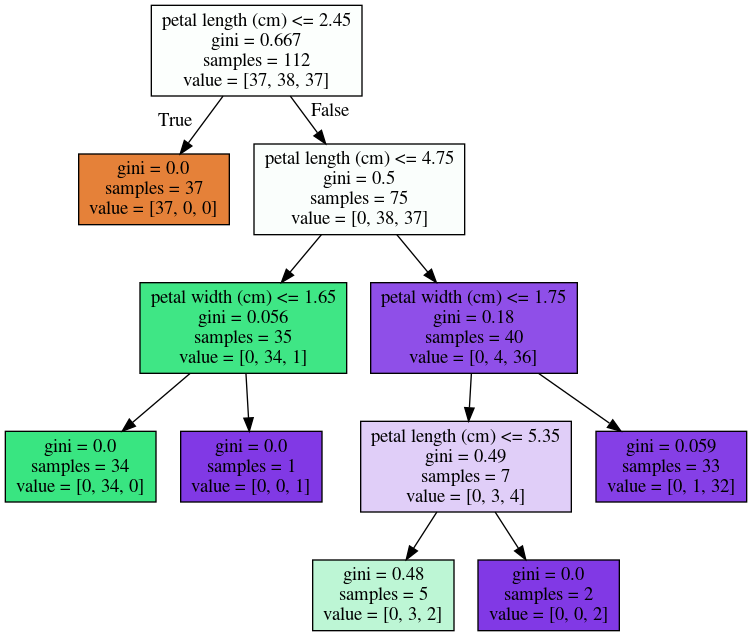
Instability
X_train, X_test, y_train, y_test = \
    train_test_split(iris.data,
                     iris.target,
                     stratify=iris.target,
                     random_state=0)
tree = DecisionTreeClassifier(max_leaf_nodes=6)
tree.fit(X_train, y_train)
X_train, X_test, y_train, y_test = \
    train_test_split(iris.data,
                     iris.target,
                     stratify=iris.target,
                     random_state=1)
tree = DecisionTreeClassifier(max_leaf_nodes=6)
tree.fit(X_train, y_train)
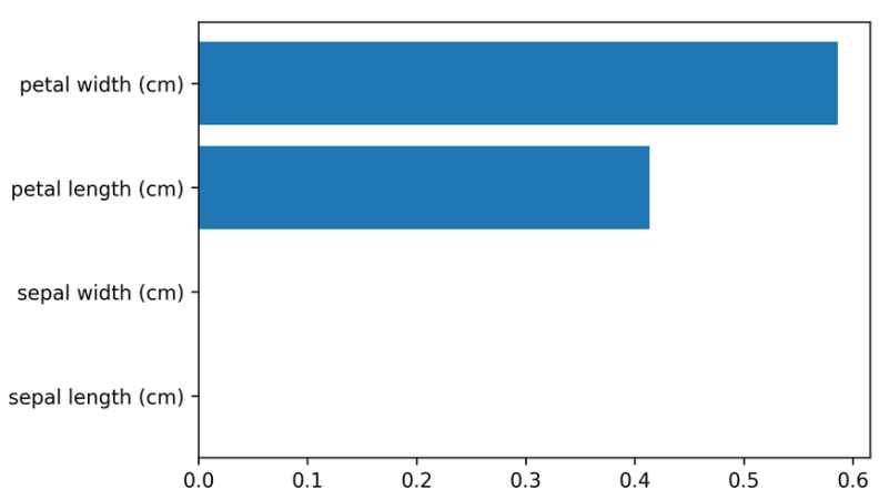
Other Tree Details
Feature importance
X_train, X_test, y_train, y_test = \
    train_test_split(iris.data,
                     iris.target,
                     stratify=iris.target,
                     random_state=1)
tree = DecisionTreeClassifier(max_leaf_nodes=6)
tree.fit(X_train,y_train)
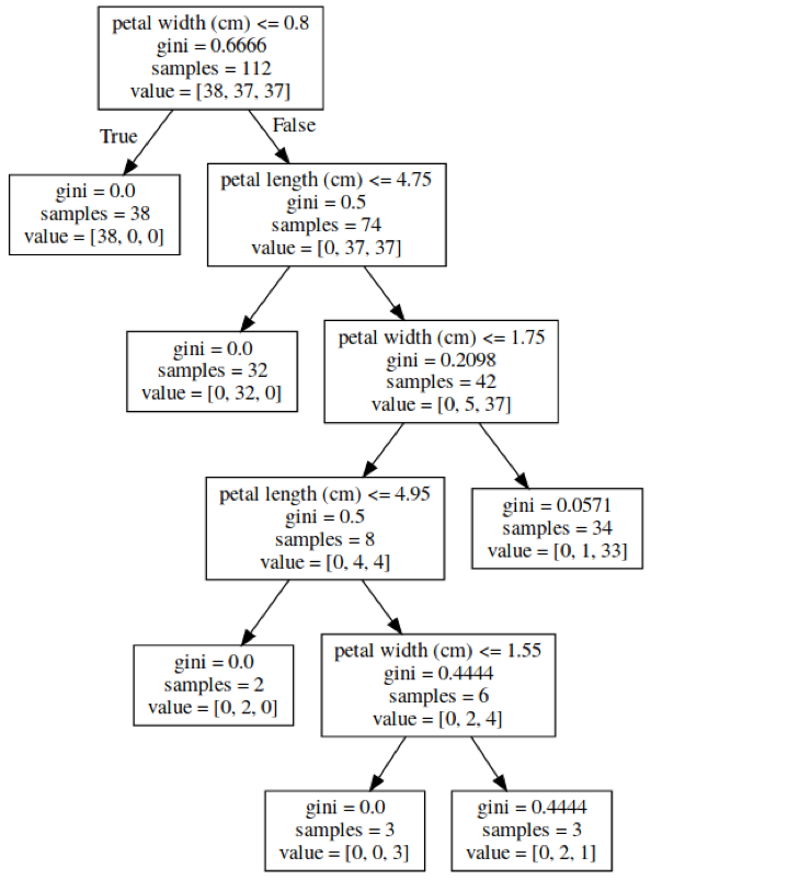
tree.feature_importances_
# array([0.0, 0.0, 0.414, 0.586])
Categorical Data
- Can split on categorical data directly (in theory)
- Intuitive way to split: split in two subsets
- \(2 ^ \text{n_values}\) many possibilities
- Possible to do in almost linear time exactly for gini index and binary classification.
- Heuristics done in practice for multi-class.
- Not in sklearn yet :(
Predicting probabilities
- Fraction of class in leaf.
- Without pruning: Always 100% certain!
- Even with pruning might be too certain.
Conditional Inference Trees
- Select "best" split with correcting for multiple-hypothesis testing.
- More "fair" to categorical variables.
- Only in R so far (
party)
Different splitting methods
 (taken from Shotton et. al. Real-Time Human Pose Recognition)