Linear Models for Classification

10/05/2022

Robert Utterback (based on slides by Andreas Muller)

\( \renewcommand{\vec}[1]{\boldsymbol{#1}} \newcommand{\E}{\mathop{\boldsymbol{E}}} \newcommand{\var}{\boldsymbol{Var}} \newcommand{\norm}[1]{\lvert\lvert#1\rvert\rvert} \newcommand{\abs}[1]{\lvert#1\rvert} \newcommand{\ltwo}[1]{\norm{#1}_2} \newcommand{\lone}[1]{\norm{#1}_1} \newcommand{\sgn}[1]{\text{sign}\left( #1 \right)} \newcommand{\e}{\mathrm{e}} \newcommand{\minw}{\min_{\vec{w} \in \mathbb{R}^p, b\in\mathbb{R}}} \newcommand{\summ}{\sum_{i=1}^m} \newcommand{\sumn}{\sum_{i=1}^n} \newcommand{\logloss}{\ln{(\exp{(-y^{(i)}(\vec{w}^T\vec{x}^{(i)}+b))} + 1)}} \)

Linear models for binary classification

\[ \hat{y} = \sgn{\vec{w}^T \vec{x} + b} = \sgn{\sum^{(i)} w^{(i)} x^{(i)} + b}\]

Similar to the regression case, basically all linear models for classification have the same way to make predictions. As with regression, they compute an inner product of a weight vector w with the feature vector x, and add some bias b. The result of that is a real number, as in regression. For classification, however, we only look at the sign of the result, so whether it is negative or positive. If it's positive, we predict one class, usually called +1, if it's negative, we predict the other class, usually called -1. If the result is 0, by convention the positive class is predicted, but because it's a floating point number that doesn't really happen in practice. You'll see that sometimes in my notation I will not have a b. That's because you can always add a constant feature to x to achieve the same effect (thought you would then need to leave that feature out of the regularization). So when I write wTx without a b assume that there is a constant feature added that is not part of any regularization (although I will try to use theta*b in that case…).

Geometrially, what the formula means is that the decision boundary of a linear classifier will be a hyperplane in the feature space, where w is the normal vector of that plane. In the 2d example here, it's just a line separating red and blue. Everything on the right hand side would be classified as blue by this classifier, and everything on the left-hand side as red.

Questions? So again, the learning here consists of finding parameters w and b based on the training set, and that is where the different algorithms differ. There are quite a lot of algorithms out there, and there are also quite a lot in scikit-learn, but we'll only discuss the most common ones.

The most straight-forward way to approach finding w and b is to use the framework of empirical risk minimization that we talked about last time, so finding parameters that minimize some loss of the training set. Where classification differs quite a bit from regression is on how we want to measure misclassifications.

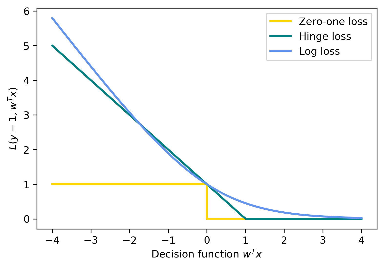
Loss Functions

\[ \hat{y} = \sgn{\vec{w}^T\vec{x} + b}\] \[ \min_{\vec{w} \in \mathbb{R}^p} \sum_{i=1}^m \mathbf{1}_{\{ y^{(i)} \ne \sgn{w^T\vec{x}^{(i)} + b} \}} \]

So we need to define a loss function for given w and b that tell us how well they fit the training set. Obvious Idea: Minimize number of misclassifications aka 0-1 loss but this loss is non-convex, not continuous and minimizing it is NP-hard. So we need to relax it, which basically means we want to find a convex upper bound for this loss. This is not done on the actual prediction, but on the inner product wTx, which is also called the decision function. So this graph here has the inner product on the x axis, and shows what the loss would be for class 1. The 0-1 loss is zero if the decision function is positive, and one if it's negative. Because a positive decision function means a positive predition, means correct classification in the case of y=1. A negative prediction means a wrong classification, which is penalized by the 0-1 loss with a loss of 1, i.e. one mistake.

The other losses we'll talk about are mostly the hinge loss and the log loss. You can see they are both upper bounds on the 0-1 loss but they are convex and continuous. Both of these losses care not only that you make a correct prediction, but also "how correct" your prediction is, i.e. how positive or negative your decision function is. We'll talk a bit more about the motivation of these two losses, starting with the logistic loss.

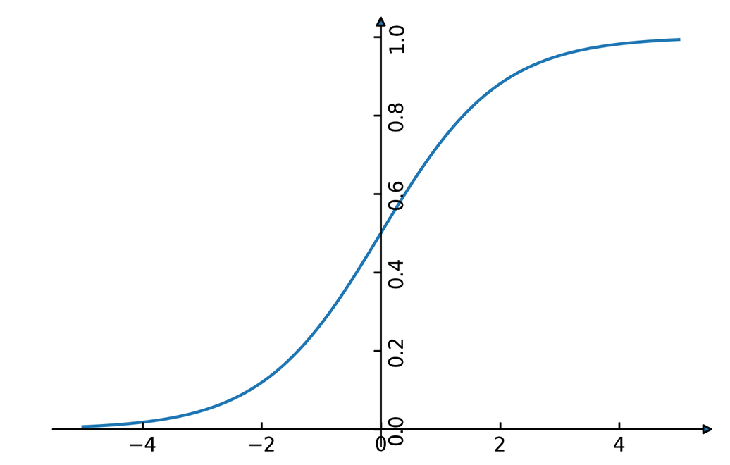
Logistic Regression

\[ \ln\left( \frac{p(y=1 | \vec{x})}{p(y=0 | \vec{x})} \right) = \vec{w}^T \vec{x} \] \[ p(y | \vec{x}) = \frac{1}{1 + \e^{-\vec{w}^T\vec{x}-b}} \] \[ \minw \sum_{i=1}^m \ln{(\exp{(-y^{(i)}\vec{w}^T\vec{x}^{(i)}+b)} + 1)} \] \[ \hat{y} = \sgn{\vec{w}^T\vec{x} + b} \]

Logistic regression is probably the most commonly used linear classifier, maybe the most commonly used classifier overall. The idea is to model the log-odds (logit), which is log p(y=1|x) - log p(y=0|x) as a linear function, as shown here. Rearranging the formula, you get a model of p(y=1|x) as 1 over 1 + … This function is called the logistic sigmoid, and is drawn to the right here. Basically it squashed the linear function wTx between 0 and 1, so that it can model a probability.

Given this equation for p(y|x), what we want to do is maximize the probability of the training set under this model. This approach is known as maximum likelihood. Basically you want to find w and b such that they assign maximum probability to the labels observed in the training data. You can rearrange that a bit and end up with this equation here, which contains the log-loss as seen on the last slide. Notice that because we're using y=1 or y=-1, we directly use yi here in a different way than the book.

The prediction is the class with the higher probability. In the binary case, that's the same as asking whether the probability of class 1 is bigger or smaller than .5. And as you can see from the plot of the logistic sigmoid, the probability of the class +1 is greater than .5 exactly if the decision function wTx is greater than 0. So predicting the class with maximum probability is the same as predicting which side of the hyperplane given by w we are on.

Ok so this is logistic regression. We minimize this loss and get a w which defines a hyper plane. But if you think back to last time, this is only part of what we want. This formulation tries to fit the training data, but it doesn't care about finding a simple solution.

Penalized Logistic Regression

\[ \minw C \summ \logloss + \ltwo{\vec{w}}^2 \] \[ \minw C \summ \logloss + \lone{\vec{w}} \]

Penalized Logistic Regression

\[ \minw C \summ \logloss + \ltwo{\vec{w}}^2 \] \[ \minw C \summ \logloss + \lone{\vec{w}} \]

\(C\) is inverse to \(\alpha\) (or \(\frac{\alpha}{n}\))
Both versions strongly convex, l2 version smooth (differentiable).
All points contribute to w

Here I used a slightly different notation as last time, though. I'm not using alpha to multiply the regularizer, instead I'm using C to multiply the loss. That's mostly because that's how it's done in scikit-learn and it has only historic reasons. The idea is exactly the same, only now C is 1 over alpha. So large C means heavy weight to the loss, means little regularization, while small C means less weight on the loss, means strong regularization.

Depending on the model, there might be a factor of n_samples in there somewhere. Usually we try to make the objective as independent of the number of samples as possible in scikit-learn, but that might lead to surprises if you're not aware of it.

Some side-notes on the optimization problem: here, as in regression, having more regularization makes the optimization problem easier. You might have seen this in your homework already, if you decrease C, meaning you add more regularization, your model fits more quickly.

One particular property of the logistic loss, compared to the hinge loss we'll discuss next is that each data point contributes to the loss, so each data point has an effect on the solution. That's also true for all the regression models we saw last time.

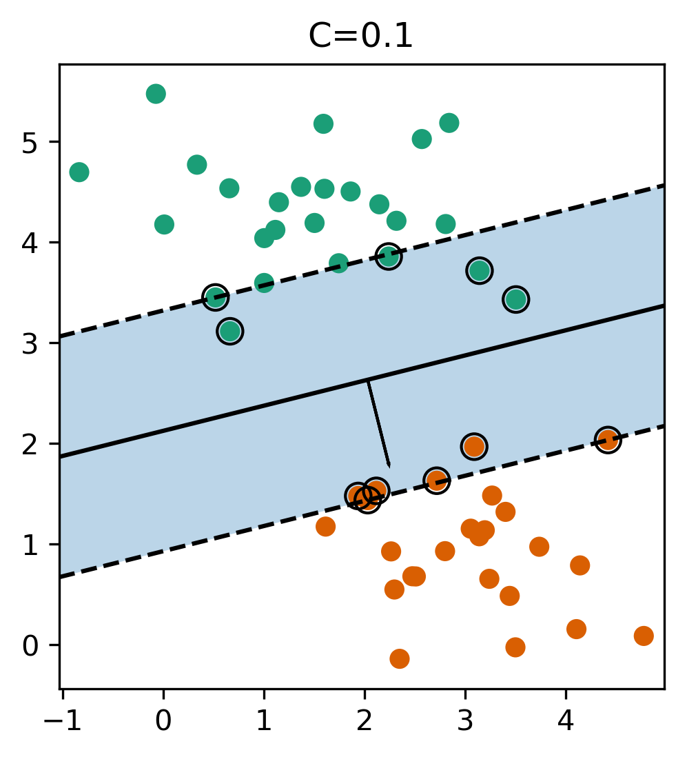
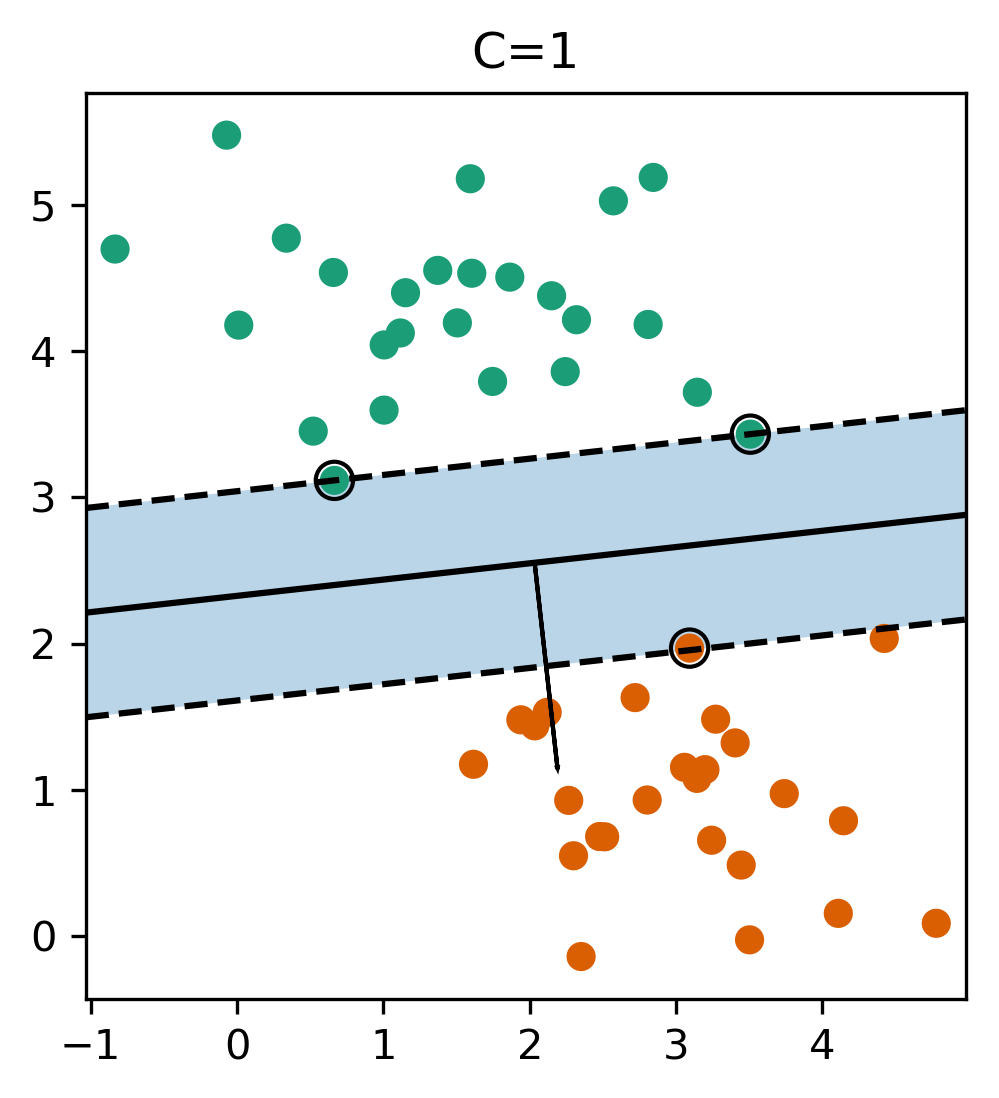
Effect of Regularization

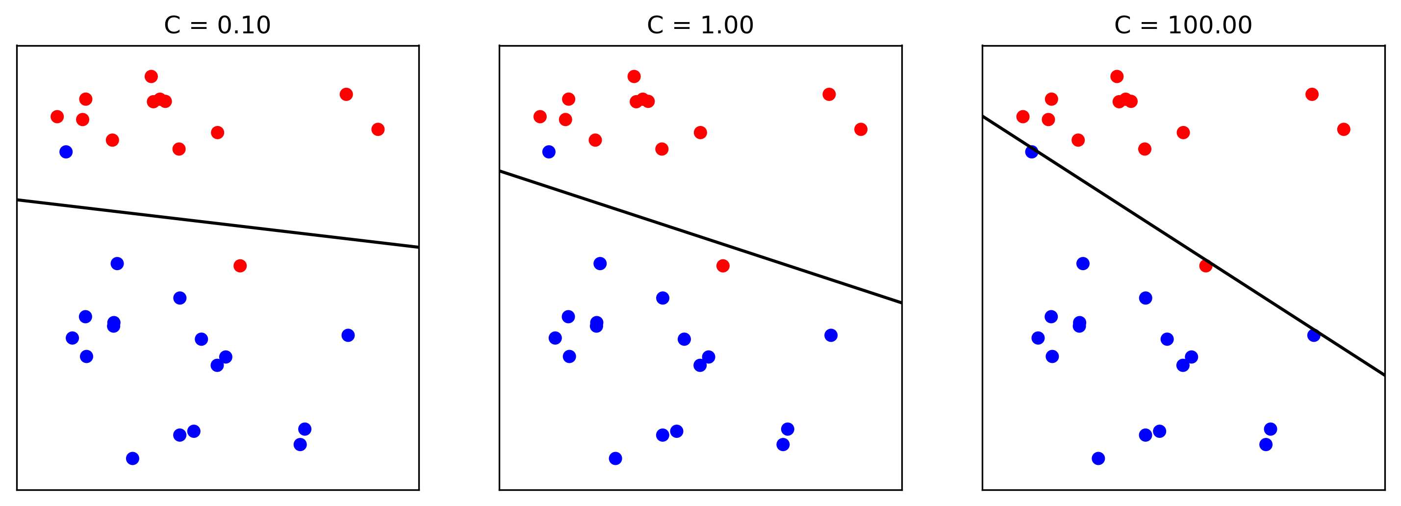
Small C limits influence of individual points.

So I spared you with coefficient plots, because they looks the same as for regression. All the things I said about model complexity and dependency on the number of features and samples is as true for classification as it is for regression.

There is another interesting way to thing about regularization that I found helpful, though. I'm not going to walk through the math for this, but you can reformulate the optimization problem and find that what the C parameter does is actually limit the influence of individual data points. With very large C, we said we have no regularization. It also means individual data points can have basically unlimited influence, as you can see here. There are two outliers here, which basically completely tilt the decision boundary. But if we decrease C, and therefore increase the regularization, what happens is that the influence of these outlier points becomes limited, and the other points get more influence.

Support Vector Machines

Max-Margin and Support Vectors

Max Margin and Support Vectors

\[ \minw C \summ \max(0, 1-y^{(i)}(\vec{w}^T \vec{x}^{(i)}+b)) + \ltwo{\vec{w}}^2 \] \[ \minw C \summ \max(0, 1-y^{(i)}(\vec{w}^T \vec{x}^{(i)}+b)) + \lone{\vec{w}} \]

Within margin \(\iff y \vec{w}^T \vec{x} < 1\)
Smaller \(\vec{w} \implies\) larger margin

Max Margin and Support Vectors

max_margin_C_0.1.png

Here are two examples on the same dataset where Andreas trained linear support vector machine with c=0.1, and c=1. With c=0.1, you have a wider margin. There are points inside the margin and all the points inside the margin are support vectors which contribute to the solution. Points that are outside of the margin and on the correct side doesn't contribute to the solution. These points are sort of classified correctly, not when they’re ignored. The normal vector is w and basically, the size of the margin is the inverse of the length of w. C=0.1 means I have less emphasis on the data fitting and more emphasis on the shrinking w. This will lead to a smaller w (thus larger margin). If I have larger C that means less regularization, which will lead to a larger W, larger W means a smaller margin. So there are fewer points here, they are inside the margin and therefore, fewer support vectors. More regularization usually means a larger margin but more points inside the margin. Also, more support vectors mean there are more data points that actually influence the solution.

(soft margin) Linear SVM

\[ \minw C \summ \max(0, 1-y^{(i)}(\vec{w}^T \vec{x}^{(i)}+b)) + \ltwo{\vec{w}}^2 \] \[ \minw C \summ \max(0, 1-y^{(i)}(\vec{w}^T \vec{x}^{(i)}+b)) + \lone{\vec{w}} \]

Both versions strongly convex, neither smooth.
Only some points contribute (the support vectors) to \(\vec{w}\)

Moving from logistic regression to linear SVMs is just a matter of changing the loss from the log loss to the hinge loss. The hinge-loss is defined as … And we can penalize using either l1 or l2 norm, or again, in principle also elastic net. This formulation with the hinge loss doesn't really make sense without the penalty, because of the formulation of the hinge loss. What this loss says is basically "if you predict the right class with a margin of 1, there is no loss". Otherwise the loss is linear in the decision function. So you need to be on the right side of the hyperplane by a given amount, and then there is no more loss. That's the reason you need the penalty, for the 1 to make sense. Otherwise you could just scale up w to make it far enough on the right side. But the regularization penalizes growing w.

The hinge loss has a kink, same as the l1 norm, and so it's not a smooth optimization problem any more, but that's not really a big deal. What's interesting is that all the points that are classified correctly with a margin of at least 1 have a loss of zero, and so they don't influence the solution any more. All the points that are not classified correctly by this margin are the ones that do influence the solution and they are called the support vectors.

Logistic Regression vs. SVM

\[ \minw C \summ \logloss + \ltwo{\vec{w}}^2 \] \[ \minw C \summ \max(0, 1-y^{(i)}(\vec{w}^T \vec{x}^{(i)}+b)) + \ltwo{\vec{w}}^2 \]

When to Use

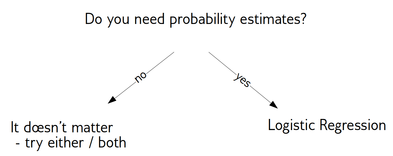
Need compact model or believe solution is sparse? Use l1.

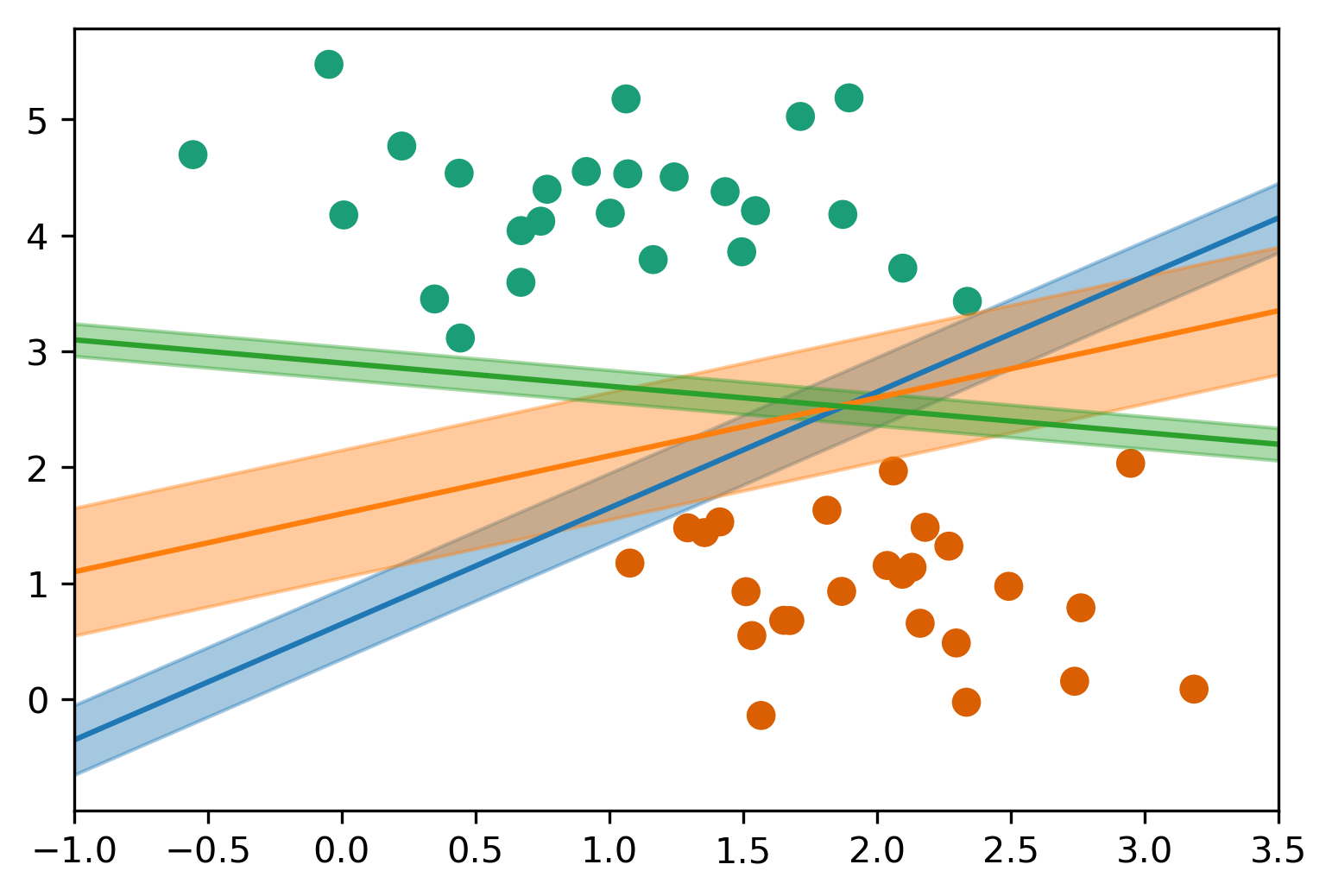
Multiclass Classification

Multinomial Logistic Regression

\[ p(y=i | \vec{x}) = \frac{\e^{(\vec{w}^{(i)})^T \vec{x} + b^{(j)}}}{\sum_{j=1}^k \e^{(\vec{w}^{(j)})^T \vec{x} + b^{(j)}}} \] \[ \min_{\vec{w}\in\mathbb{R}^{pk},b\in\mathbb{R}^k} \sum_{i=1}^m \ln(p(y=y^{(i)} | x^{(i)})) \] \[ \hat{y} = \text{argmax}_{i \in 1,\ldots,k} ((\vec{w}^{(i)})^T \vec{x} + b^{(i)}) \]

Same prediction rule as OVR.

In scikit-learn

OVO: Only option for SVC
OVR: default for all linear models except LogisticRegression
clf.decision_function \(=\vec{w}^T \vec{x}\)
clf.predict_proba gives probabilities for each class
SVC(probability=True) not great

Multiclass in Practice

iris = load_iris()
X,y = iris.data, iris.target
print(X.shape)
print(np.bincount(y))

logreg = LogisticRegression(multi_class="multinomial",
                            random_state=0,
                            solver="lbfgs").fit(X,y)
linearsvm = LinearSVC().fit(X,y)
print(logreg.coef_.shape)
print(linearsvm.coef_.shape)

(150, 4)
[50 50 50]
(3, 4)
(3, 4)

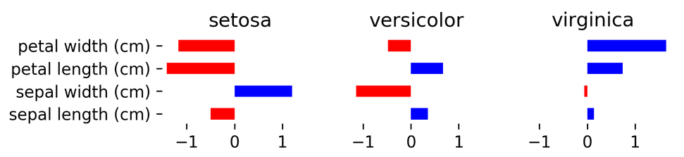
print(logreg.coef_)

[[-0.41815181  0.96640966 -2.52143555 -1.08402204]
 [ 0.53103513 -0.31447032 -0.19924552 -0.94919389]
 [-0.11288332 -0.65193934  2.72068108  2.03321592]]

Computational Considerations

(for linear models)

Solver choices

Don't use SVC(kernel='linear'), use LinearSVC
When \(p >> m\): Lars (or LassoLars) instead of Lasso
For small \(m\) (\(< 10,000\)), don't worry — it will be fast enough
LinearSVC, LogisticRegression when \(m >> p\): dual=False
LogisticRegression(solver="sag") when \(m\) is really big (100,000+)
Stochastic Gradient Descent also good when \(m\) is large