Calibration & Class Imbalance

09/19/2022

Robert Utterback (based on slides by Andreas Muller)

\( \renewcommand{\vec}[1]{\boldsymbol{#1}} \newcommand{\E}{\mathop{\boldsymbol{E}}} \newcommand{\var}{\boldsymbol{Var}} \newcommand{\norm}[1]{\lvert\lvert#1\rvert\rvert} \newcommand{\abs}[1]{\lvert#1\rvert} \newcommand{\ltwo}[1]{\norm{#1}_2} \newcommand{\lone}[1]{\norm{#1}_1} \newcommand{\sgn}[1]{\text{sign}\left( #1 \right)} \newcommand{\e}{\mathrm{e}} \newcommand{\minw}{\min_{w \in \mathbb{R}^p}} \newcommand{\sumn}{\sum_{i=1}^n} \newcommand{\logloss}{\log{(\exp{(-y_iw^T\vec{x}_i)} + 1)}} \)

Calibration

Probabilities can be much more informative than labels:
"The model predicted you don’t have cancer" vs "The model predicted you’re 40% likely to have cancer"

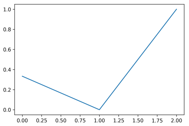
Calibration curve (Reliability diagram)

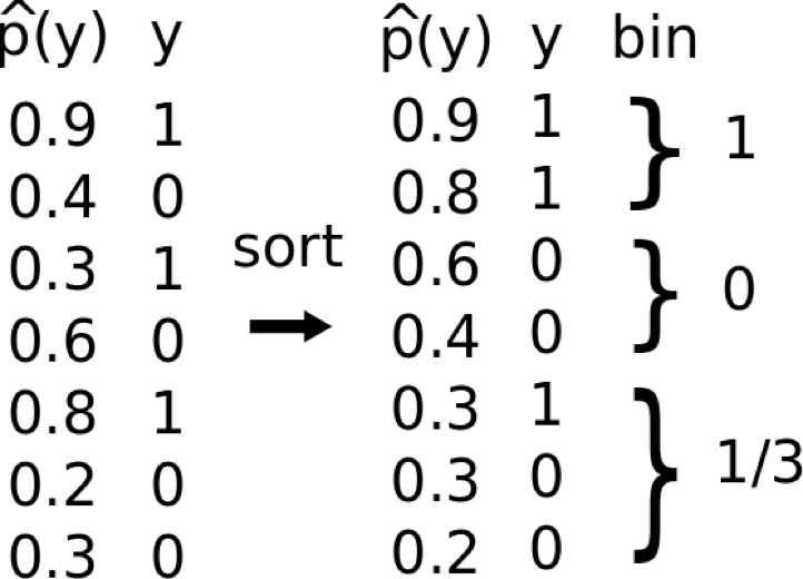
`calibration_curve` with sklearn

Using subsample of covertype dataset

from sklearn.linear_model import LogisticRegressionCV
print(X_train.shape)
print(np.bincount(y_train))
lr = LogisticRegressionCV().fit(X_train, y_train)
# (52292, 54)
# [19036 33256]

lr.C_
array([ 2.783])

print(lr.predict_proba(X_test)[:10])
print(y_test[:10])
# [[ 0.681  0.319]
#  [ 0.049  0.951]
#  [ 0.706  0.294]
#  [ 0.537  0.463]
#  [ 0.819  0.181]
#  [ 0.     1.   ]
#  [ 0.794  0.206]
#  [ 0.676  0.324]
#  [ 0.727  0.273]
#  [ 0.597  0.403]]
# [0 1 0 1 1 1 0 0 0 1]

from sklearn.calibration import calibration_curve
probs = lr.predict_proba(X_test)[:, 1]
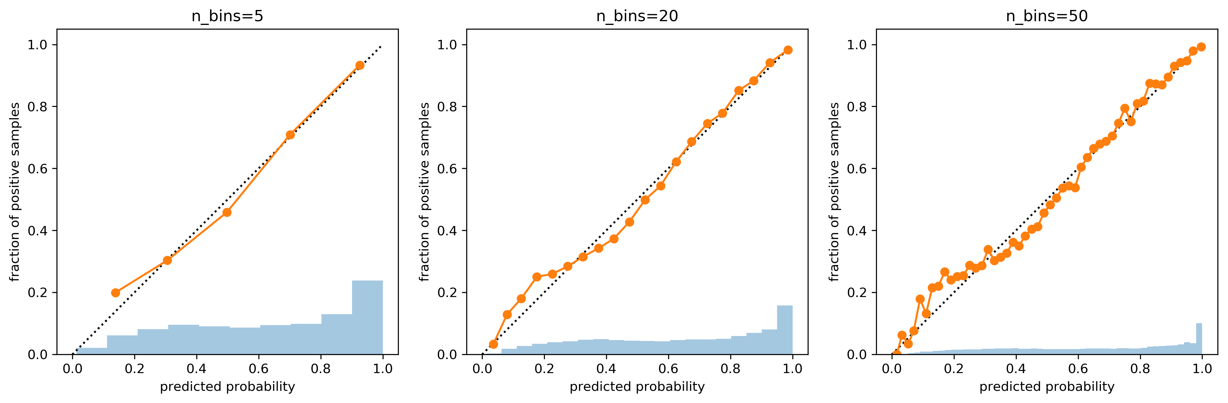
prob_true, prob_pred = calibration_curve(y_test, probs, n_bins=5)
print(prob_true)
print(prob_pred)
# [ 0.2    0.303  0.458  0.709  0.934]
# [ 0.138  0.306  0.498  0.701  0.926]

Influence of number of bins

Comparing Models

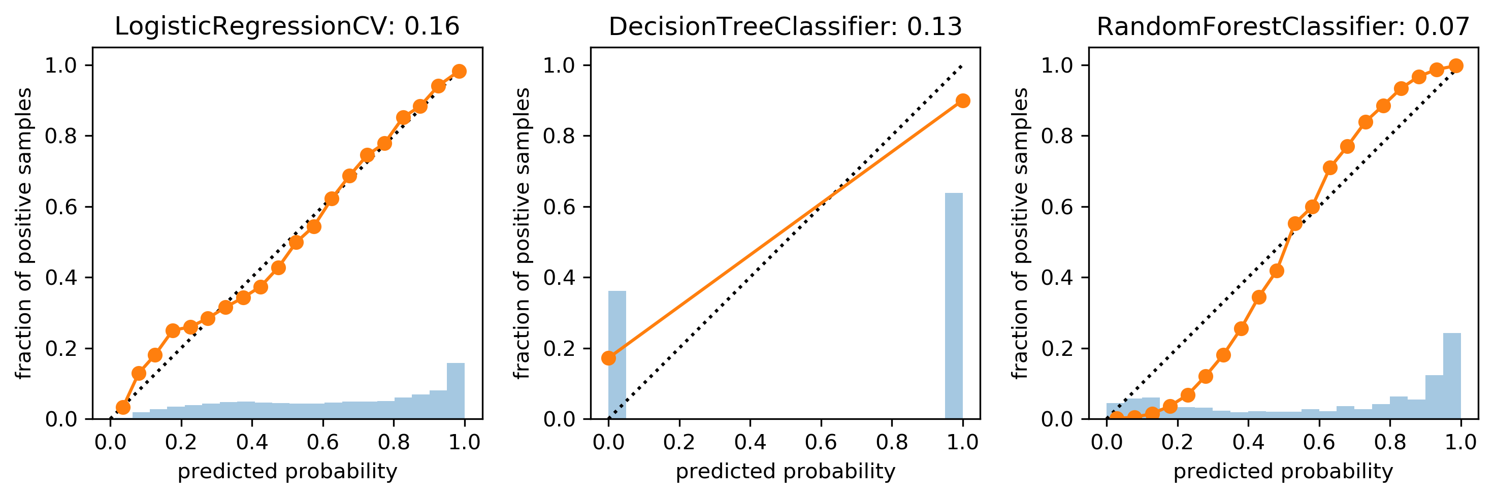
Brier Score (for binary classification)

"mean squared error of probability estimate"

\[ BS = \frac{\sum_{i=1}^{n} (\widehat{p} (y_i)-y_i)^{2}}{n}\]

Fixing it: Calibrating a classifier

Build another model, mapping classifier probabilities to better probabilities!
1d model! (or more for multi-class)

\[ f_{callib}(s(x)) \approx p(y)\]

s(x) is score given by model, usually
Can also work with models that don’t even provide probabilities! Need model for \(f_{callib}\), need to decide what data to train it on.
Can train on training set \(\to\) Overfit
Can train using cross-validation \(\to\) use data, slower

Platt Scaling

Use a logistic sigmoid for \(f_{callib}\)
Basically learning a 1d logistic regression
(+ some tricks)
Works well for SVMs

\[f_{platt} = \frac{1}{1 + exp(-ws(x))}\]

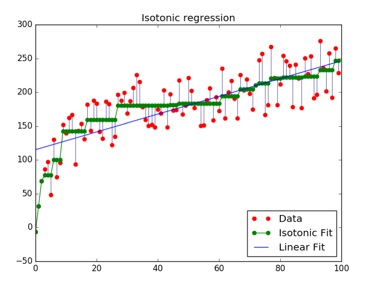
Isotonic Regression

Very flexible way to specify \(f_{callib}\)
Learns arbitrary monotonically increasing step-functions in 1d.
Groups data into constant parts, steps in between.
Optimum monotone function on training data (wrt mse).

Building the model

Using the training set is bad
Either use hold-out set or cross-validation
Cross-validation can be use as in stacking to make unbiased probability predictions, use that as training set.

CalibratedClassifierCV

from sklearn.calibration import CalibratedClassifierCV
X_train_sub, X_val, y_train_sub, y_val = \
    train_test_split(X_train, y_train,
                     stratify=y_train, random_state=0)
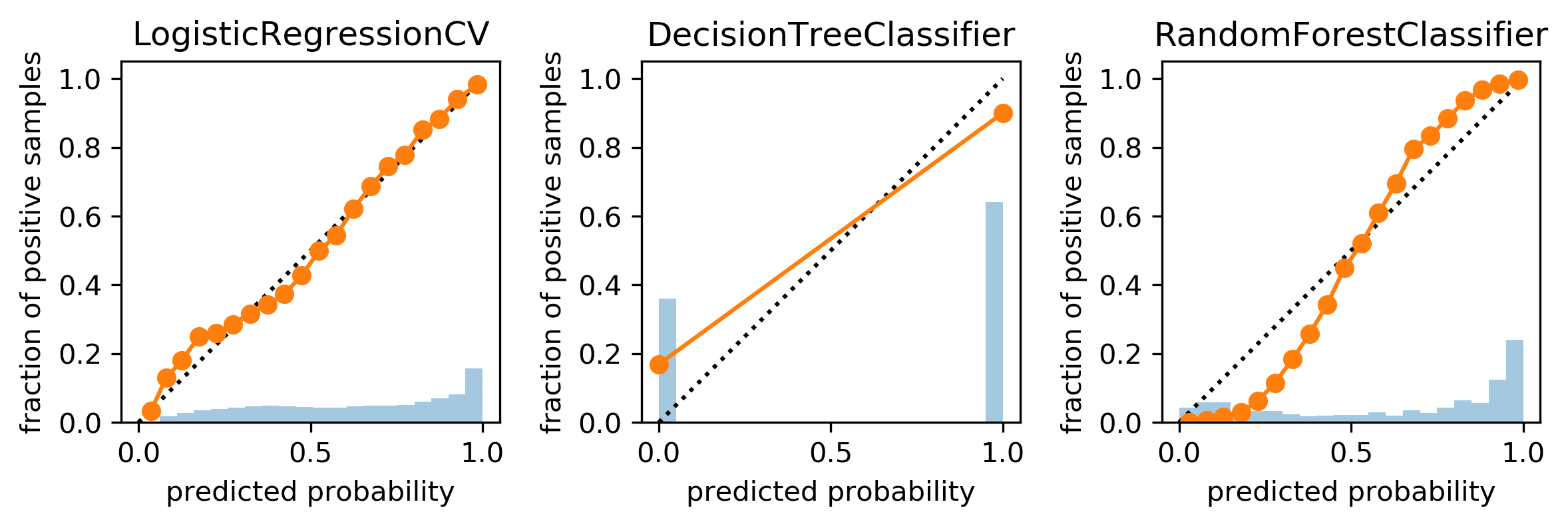
rf = RandomForestClassifier(n_estimators=100).fit(X_train_sub, y_train_sub)
scores = rf.predict_proba(X_test)[:, 1]
plot_calibration_curve(y_test, scores, n_bins=20)

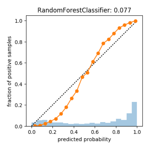
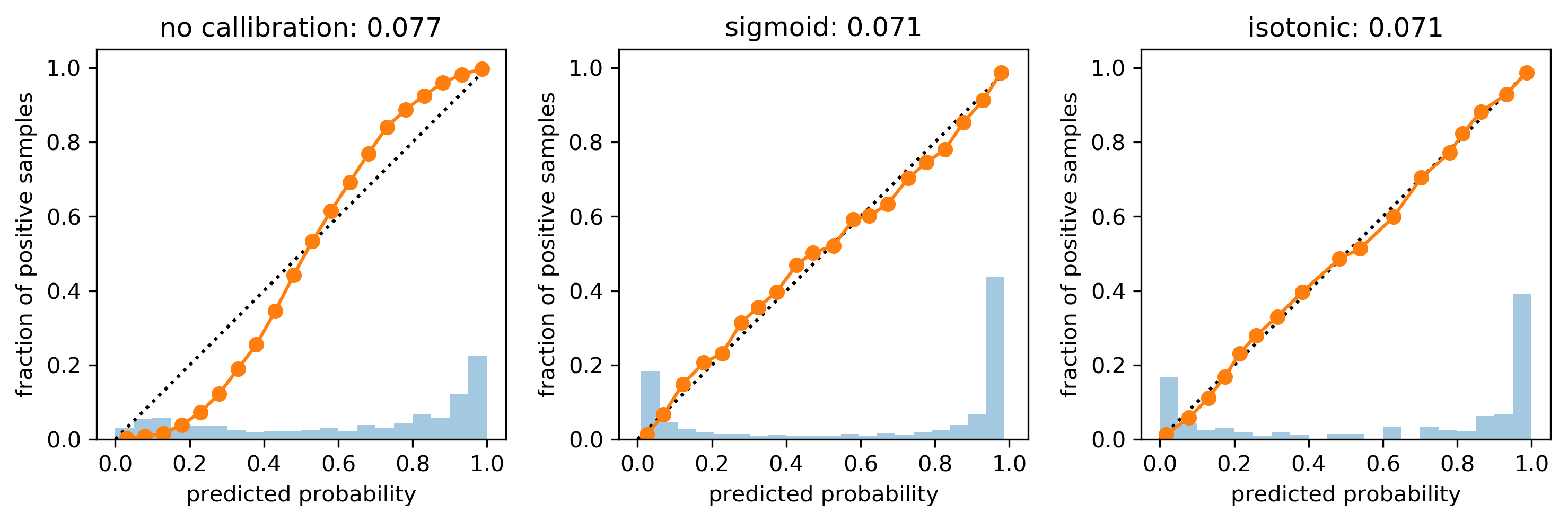
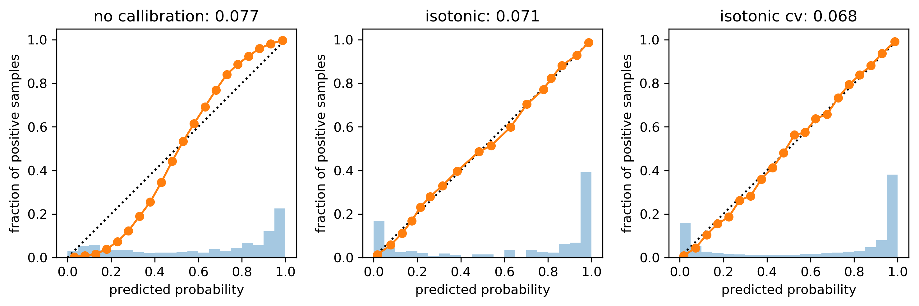
Calibration on Random Forest

cal_rf = CalibratedClassifierCV(rf, cv="prefit",
                                method='sigmoid')
cal_rf.fit(X_val, y_val)
scores_sigm = cal_rf.predict_proba(X_test)[:, 1]

cal_rf_iso = CalibratedClassifierCV(rf, cv="prefit",
                                    method='isotonic')
cal_rf_iso.fit(X_val, y_val)
scores_iso = cal_rf_iso.predict_proba(X_test)[:, 1]

Cross-validated Calibration

cal_rf_iso_cv = CalibratedClassifierCV(rf, method='isotonic')
cal_rf_iso_cv.fit(X_train, y_train)
scores_iso_cv = cal_rf_iso_cv.predict_proba(X_test)[:, 1]

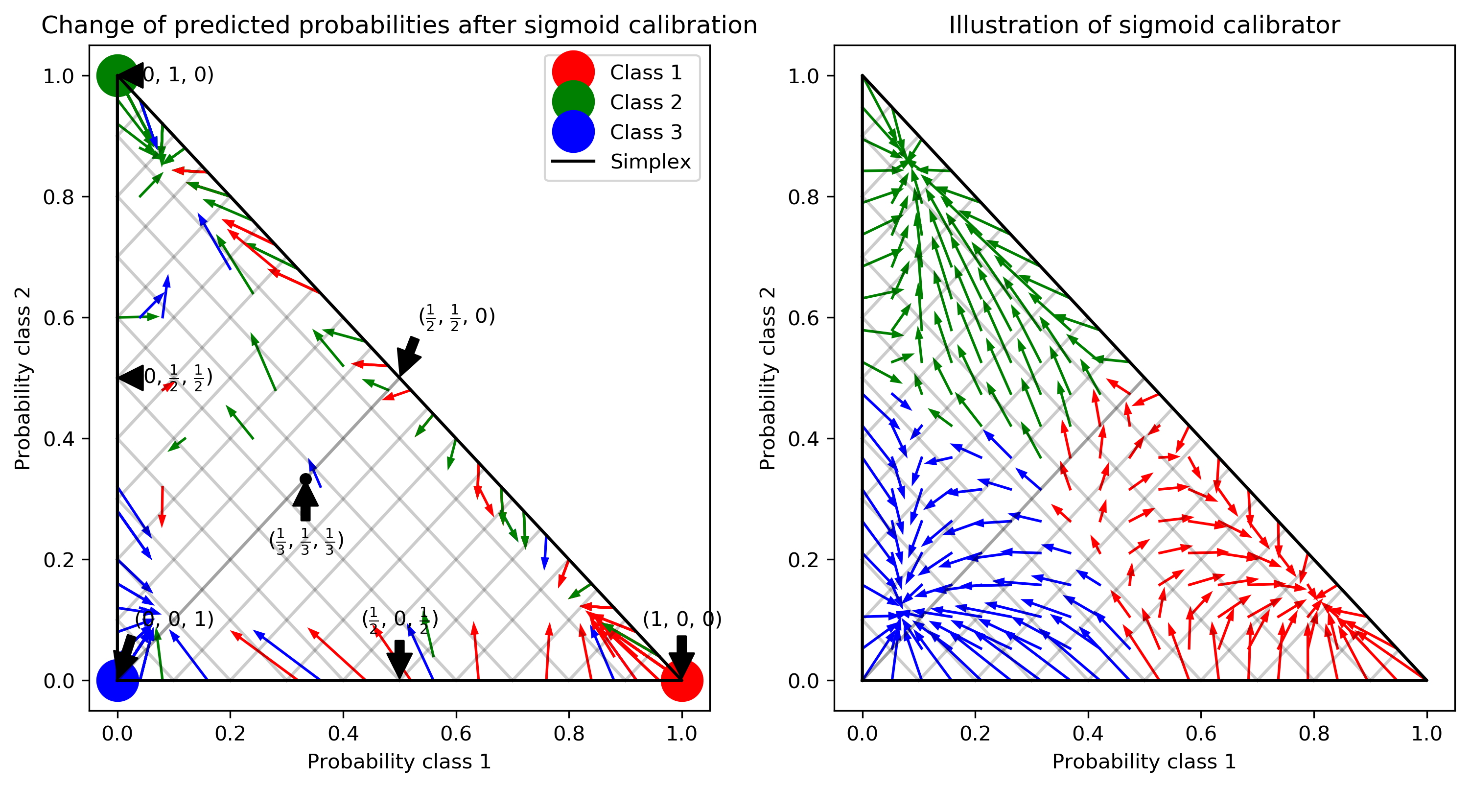
Multi-Class Calibration

Class Imbalance

Two sources of imbalance

Asymmetric cost
Asymmetric data

Why do we care?

Why should cost be symmetric?
All data is imbalanced
Detect rare events

Changing Thresholds

data = load_breast_cancer()
lr = LogisticRegression(solver='lbfgs', max_iter=10000)
X_train, X_test, y_train, y_test = \
    train_test_split(data.data, data.target,
                     stratify=data.target, random_state=0)

lr.fit(X_train, y_train)
y_pred = lr.predict(X_test)

print(classification_report(y_test, y_pred))

              precision    recall  f1-score   support

           0       0.91      0.92      0.92        53
           1       0.96      0.94      0.95        90

    accuracy                           0.94       143
   macro avg       0.93      0.93      0.93       143
weighted avg       0.94      0.94      0.94       143

y_pred = lr.predict_proba(X_test)[:, 1] > .85

print(classification_report(y_test, y_pred))

              precision    recall  f1-score   support

           0       0.84      1.00      0.91        53
           1       1.00      0.89      0.94        90

    accuracy                           0.93       143
   macro avg       0.92      0.94      0.93       143
weighted avg       0.94      0.93      0.93       143

roc curve

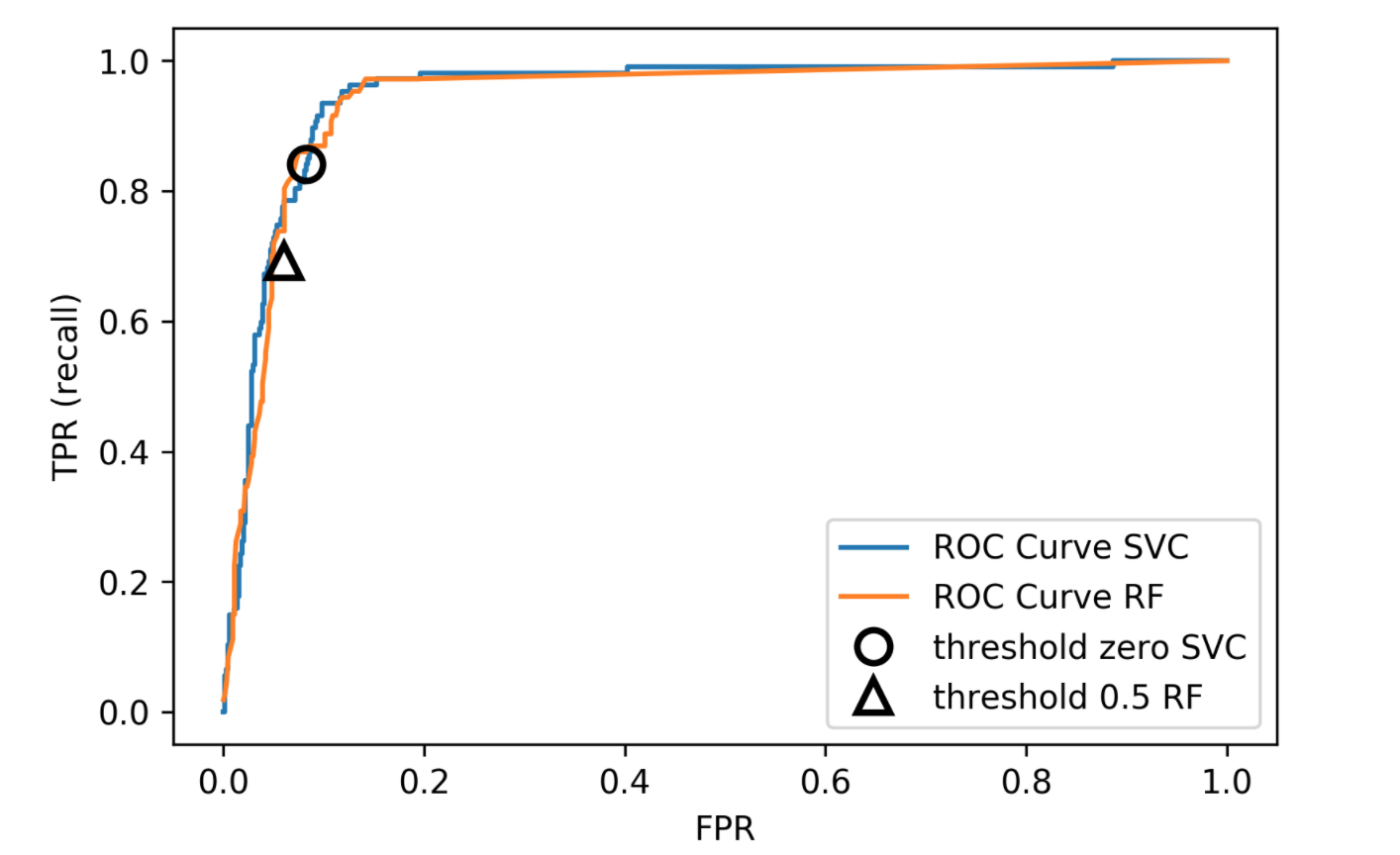
remedies for the model

Mammography Data

from sklearn.datasets import fetch_openml
data = fetch_openml('mammography', as_frame=True)
X, y = data.data, data.target
print(X.shape)

(11183, 6)

print(y.value_counts())

-1    10923
1       260
Name: class, dtype: int64

Mammography Data

lr = LogisticRegression(solver='lbfgs')
scores = cross_validate(lr, X_train, y_train, cv=10,
                        scoring=('roc_auc', 'average_precision'))
roc = scores['test_roc_auc'].mean()
avep = scores['test_average_precision'].mean()
print(f"{roc:.3f}, {avep:.3f}")

0.918, 0.631

rf = RandomForestClassifier(n_estimators=100)
scores = cross_validate(rf, X_train, y_train, cv=10,
                        scoring=('roc_auc', 'average_precision'))
roc = scores['test_roc_auc'].mean()
avep = scores['test_average_precision'].mean()
print(f"{roc:.3f}, {avep:.3f}")

0.943, 0.738

Mammography Data

Basic Approaches

Change the training procedure

Change the Data: Sampling

Scikit-learn vs. resampling

Imbalance-learn

http://imbalanced-learn.org

!pip install imbalanced-learn
# or conda install ...

Extends sklearn API

Sampler

To resample data sets, each sampler implements

data_resampled, targets_resampled = obj.resample(data, targets)

Fitting and sampling in one step:

data_resampled, targets_resampled = \
	obj.fit_resample(data, targets)

In pipelines: sampling only done in fit!

Random Undersampling

from imblearn.under_sampling import RandomUnderSampler
rus = RandomUnderSampler(replacement=False)
X_train_subsample, y_train_subsample = \
    rus.fit_resample(X_train, y_train)
print(X_train.shape)
print(X_train_subsample.shape)
print(np.bincount(y_train_subsample))

(8387, 6)
(392, 6)
[196 196]

Random Undersampling

from imblearn.pipeline import make_pipeline as make_imb_pipeline
undersample_pipe = make_imb_pipeline(
    RandomUnderSampler(random_state=57), lr)
scores = cross_validate(undersample_pipe,
                        X_train, y_train, cv=10,
                        scoring=('roc_auc', 'average_precision'))
roc = scores['test_roc_auc'].mean()
avep = scores['test_average_precision'].mean()
print(f"{roc:.3f}, {avep:.3f}")
# was 0.918, 0.631 without

0.921, 0.580

undersample_pipe_rf = \
    make_imb_pipeline(RandomUnderSampler(random_state=0),
                      RandomForestClassifier(n_estimators=100))
scores = cross_validate(undersample_pipe_rf,
                        X_train, y_train, cv=10, 
                        scoring=('roc_auc', 'average_precision'))
roc = scores['test_roc_auc'].mean()
avep = scores['test_average_precision'].mean()
print(f"{roc:.3f}, {avep:.3f}")
# was 0.943, 0.738 without

0.945, 0.594

Random Oversampling

from imblearn.over_sampling import RandomOverSampler
ros = RandomOverSampler(random_state=0)
X_train_oversample, y_train_oversample = \
    ros.fit_resample(X_train, y_train)
print(X_train.shape)
print(X_train_oversample.shape)
print(np.bincount(y_train_oversample))

(8387, 6)
(16382, 6)
[8191 8191]

Random Oversampling

oversample_pipe = make_imb_pipeline(
    RandomOverSampler(random_state=0), lr)

scores = cross_validate(oversample_pipe,
                        X_train, y_train, cv=10,
                        scoring=('roc_auc', 'average_precision'))
roc = scores['test_roc_auc'].mean()
avep = scores['test_average_precision'].mean()
print(f"{roc:.3f}, {avep:.3f}")
# was 0.918, 0.631 without

0.925, 0.570

oversample_pipe_rf = \
    make_imb_pipeline(RandomOverSampler(random_state=0),
                      RandomForestClassifier(n_estimators=100))
scores = cross_validate(oversample_pipe_rf,
                        X_train, y_train, cv=10,
                        scoring=('roc_auc', 'average_precision'))
roc = scores['test_roc_auc'].mean()
avep = scores['test_average_precision'].mean()
print(f"{roc:.3f}, {avep:.3f}")
# was 0.943, 0.738 without

0.923, 0.708

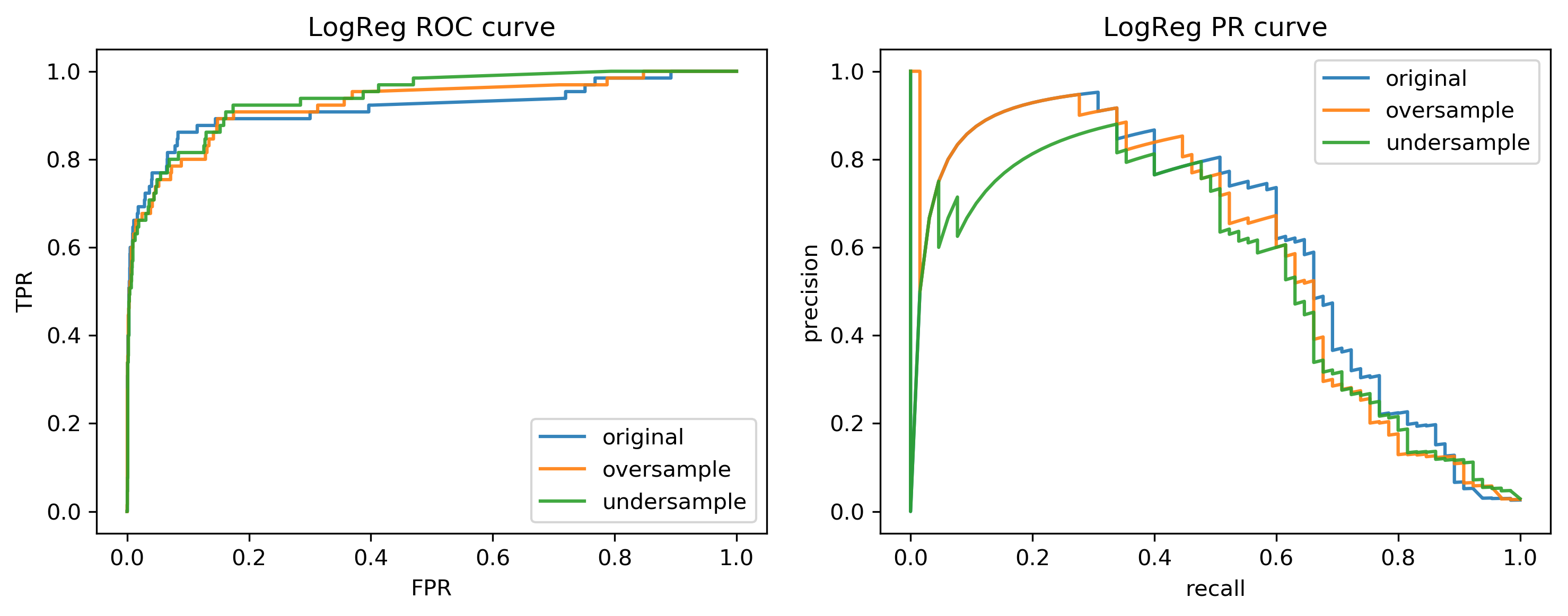
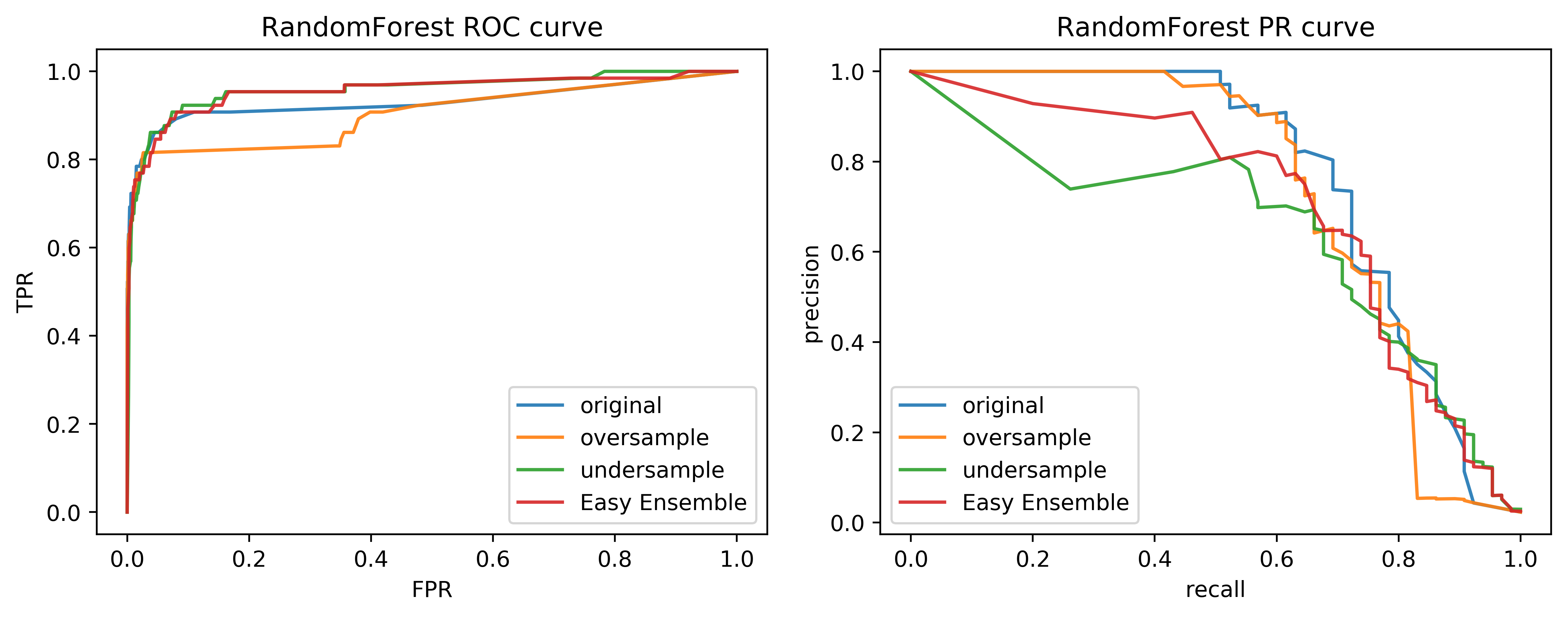
Curves for LogReg

Curves for Random Forest

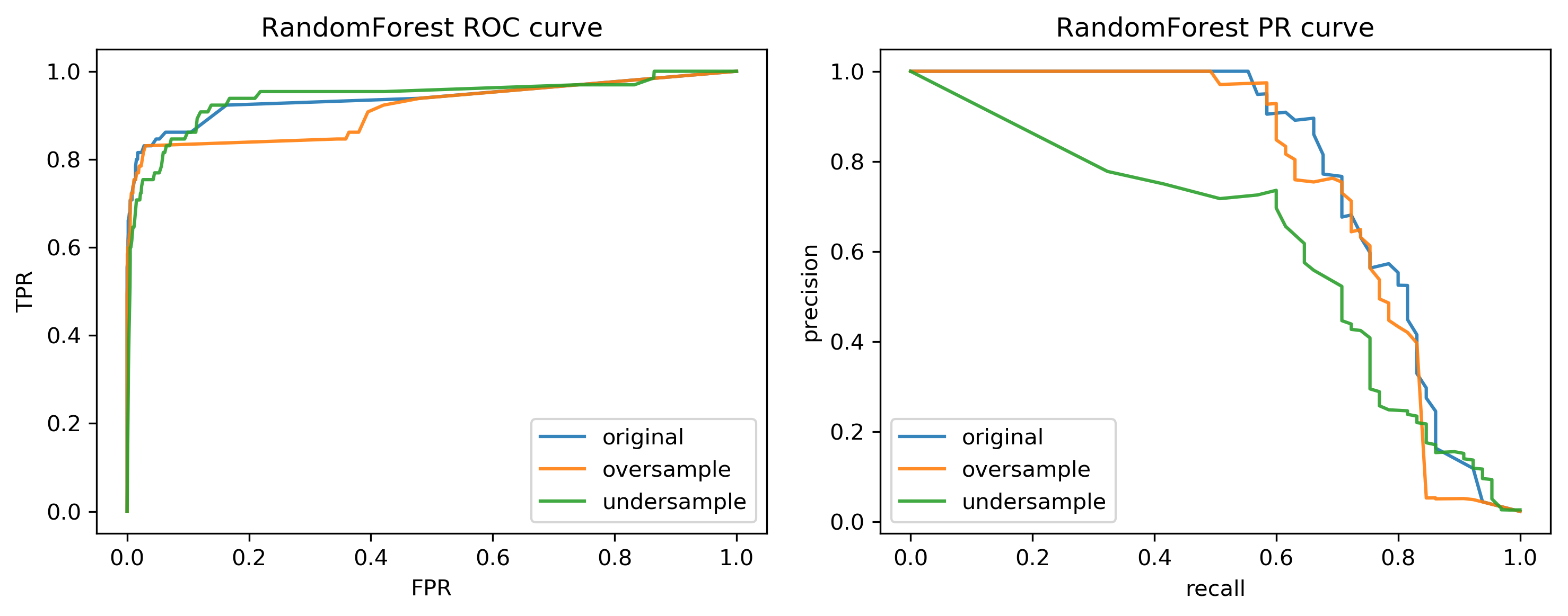
ROC or PR?

FPR or Precision? \[ \large\text{FPR} = \frac{\text{FP}}{\text{FP}+\text{TN}}\] \[ \large\text{Precision} = \frac{\text{TP}}{\text{TP}+\text{FP}}\]

Change the Training

Class-weights

Instead of repeating samples, re-weight the loss function.
Works for most models!
Same effect as over-sampling (though not random), but not as expensive (dataset size the same).

Class-weights in linear models

\[\min_{w \in ℝ^{p}}-C \sum_{i=1}^n\log(\exp(-y_iw^T \textbf{x}_i) + 1) + ||w||_2^2\] \[ \min_{w \in \mathbb{R}^p} -C \sum_{i=1}^n c_{y_i} \log(\exp(-y_i w^T \mathbf{x}_i) + 1) + ||w||^2_2 \] Similar for linear and non-linear SVM

Class weights in trees

Gini Index: \[H_\text{gini}(X_m) = \sum_{k\in\mathcal{Y}} p_{mk} (1 - p_{mk})\] \[H_\text{gini}(X_m) = \sum_{k\in\mathcal{Y}} c_k p_{mk} (1 - p_{mk})\] Prediction: Weighted vote

Using Class Weights

lr = LogisticRegression(solver='lbfgs',
                        class_weight='balanced')
scores = cross_validate(lr, X_train, y_train, cv=10,
                        scoring=('roc_auc',
                                 'average_precision'))
roc = scores['test_roc_auc'].mean()
avep = scores['test_average_precision'].mean()
print(f"{roc:.3f}, {avep:.3f}")

0.923, 0.564

rf = RandomForestClassifier(n_estimators=100,
                            class_weight='balanced')
scores = cross_validate(rf, X_train, y_train, cv=10,
                        scoring=('roc_auc',
                                 'average_precision'))
roc = scores['test_roc_auc'].mean()
avep = scores['test_average_precision'].mean()
print(f"{roc:.3f}, {avep:.3f}")


>>> 0.915, 0.707

Ensemble Resampling

Random resampling separate for each instance in an ensemble!
Paper: "Exploratory Undersampling for Class Imbalance Learning"
Not in sklearn (yet)
Easy with imblearn

Easy Ensemble with imblearn

from sklearn.tree import DecisionTreeClassifier
tree = DecisionTreeClassifier(max_features='sqrt')
from imblearn.ensemble import BalancedBaggingClassifier
resampled_rf = \
    BalancedBaggingClassifier(base_estimator=tree,
                              n_estimators=100, random_state=0)
scores = cross_validate(resampled_rf, X_train, y_train,
                        cv=10,
                        scoring=('roc_auc', 'average_precision'))
roc = scores['test_roc_auc'].mean()
avep = scores['test_average_precision'].mean()
print(f"{roc:.3f}, {avep:.3f}")

0.949, 0.668

Smart resampling

(based on nearest neighbour heuristics from the 70's)

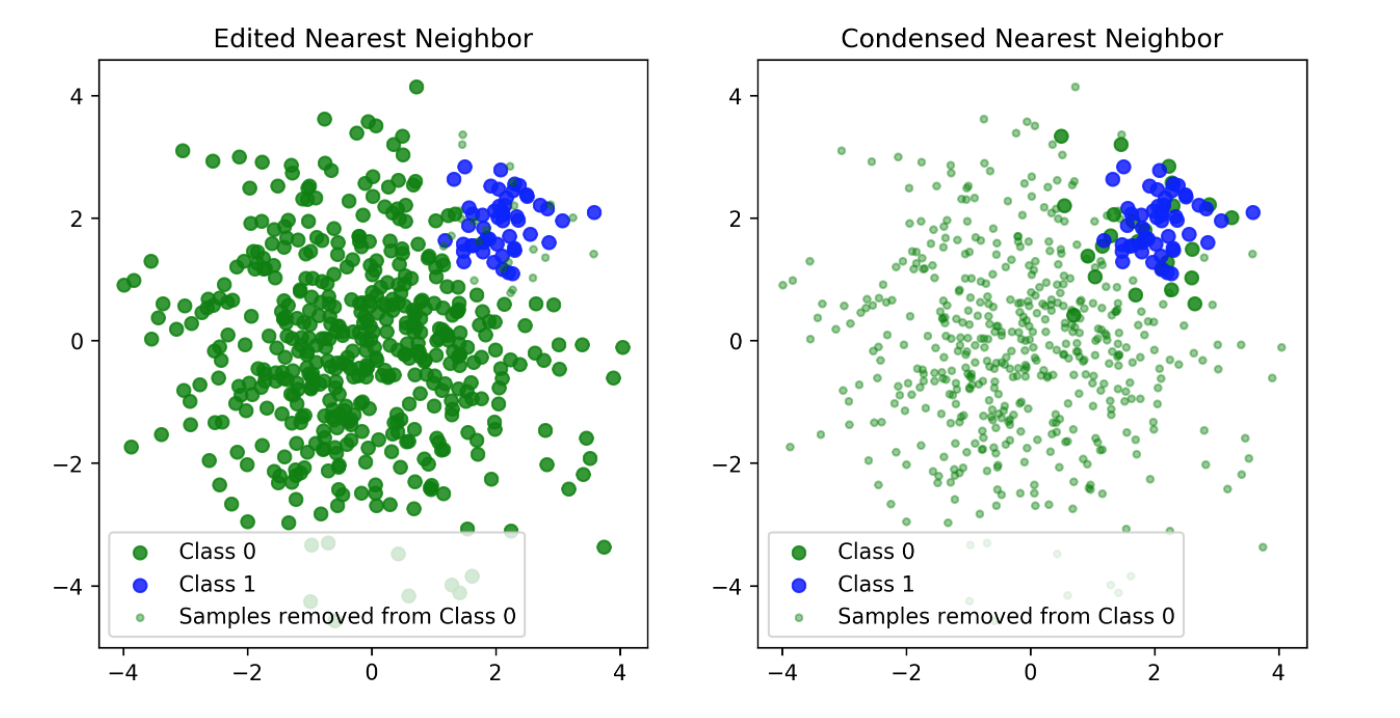
Edited Nearest Neighbours

Originally as heuristic for reducing dataset for KNN
Remove all samples that are misclassified by KNN from training data (mode) or that have any point from other class as neighbor (all).
"Cleans up" outliers and boundaries.

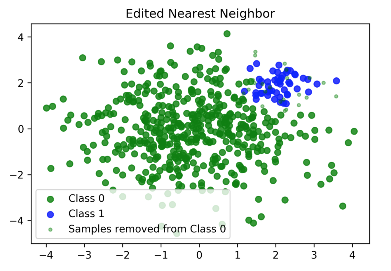
Edited Nearest Neighbours

from imblearn.under_sampling import EditedNearestNeighbours
enn = EditedNearestNeighbours(n_neighbors=5)
X_train_enn, y_train_enn = enn.fit_resample(X_train, y_train)

enn_mode = EditedNearestNeighbours(kind_sel="mode", 
                                   n_neighbors=5)
X_train_enn_mode, y_train_enn_mode = \
    enn_mode.fit_resample(X_train, y_train)

enn_pipe = make_imb_pipeline(EditedNearestNeighbours(n_neighbors=5),
                             LogisticRegression(solver='lbfgs'))
scores = cross_val_score(enn_pipe, X_train, y_train, cv=10, scoring='roc_auc')
print(f"{np.mean(scores):.3f}")

0.921

enn_pipe_rf = make_imb_pipeline(EditedNearestNeighbours(n_neighbors=5),
                                  RandomForestClassifier(n_estimators=100))
scores = cross_val_score(enn_pipe_rf, X_train, y_train, cv=10, scoring='roc_auc')
print(f"{np.mean(scores):.3f}")

0.941

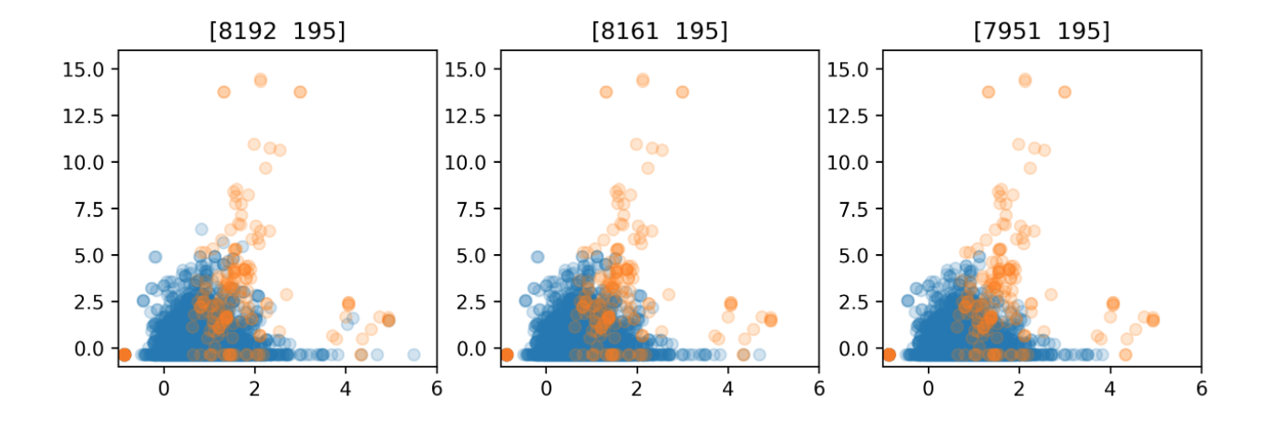
Condensed Nearest Neighbors

Iteratively adds points to the data that are misclassified by KNN
Focuses on the boundaries
Usually removes many

from imblearn.under_sampling import CondensedNearestNeighbour
cnn = CondensedNearestNeighbour()
X_train_cnn, y_train_cnn = cnn.fit_resample(X_train, y_train)
print(X_train_cnn.shape)
print(np.bincount(y_train_cnn))

(553, 6)
[357 196]

cnn_pipe = make_imb_pipeline(CondensedNearestNeighbour(),
                             LogisticRegression(solver='lbfgs'))
scores = cross_val_score(cnn_pipe, X_train, y_train, cv=10, scoring='roc_auc')
print(f"{np.mean(scores):.3f}")

0.916

rf = RandomForestClassifier(n_estimators=100, random_state=0)
cnn_pipe = make_imb_pipeline(CondensedNearestNeighbour(), rf)
scores = cross_val_score(cnn_pipe, X_train, y_train, cv=10, scoring='roc_auc')
print(f"{np.mean(scores):.2f}")

0.93

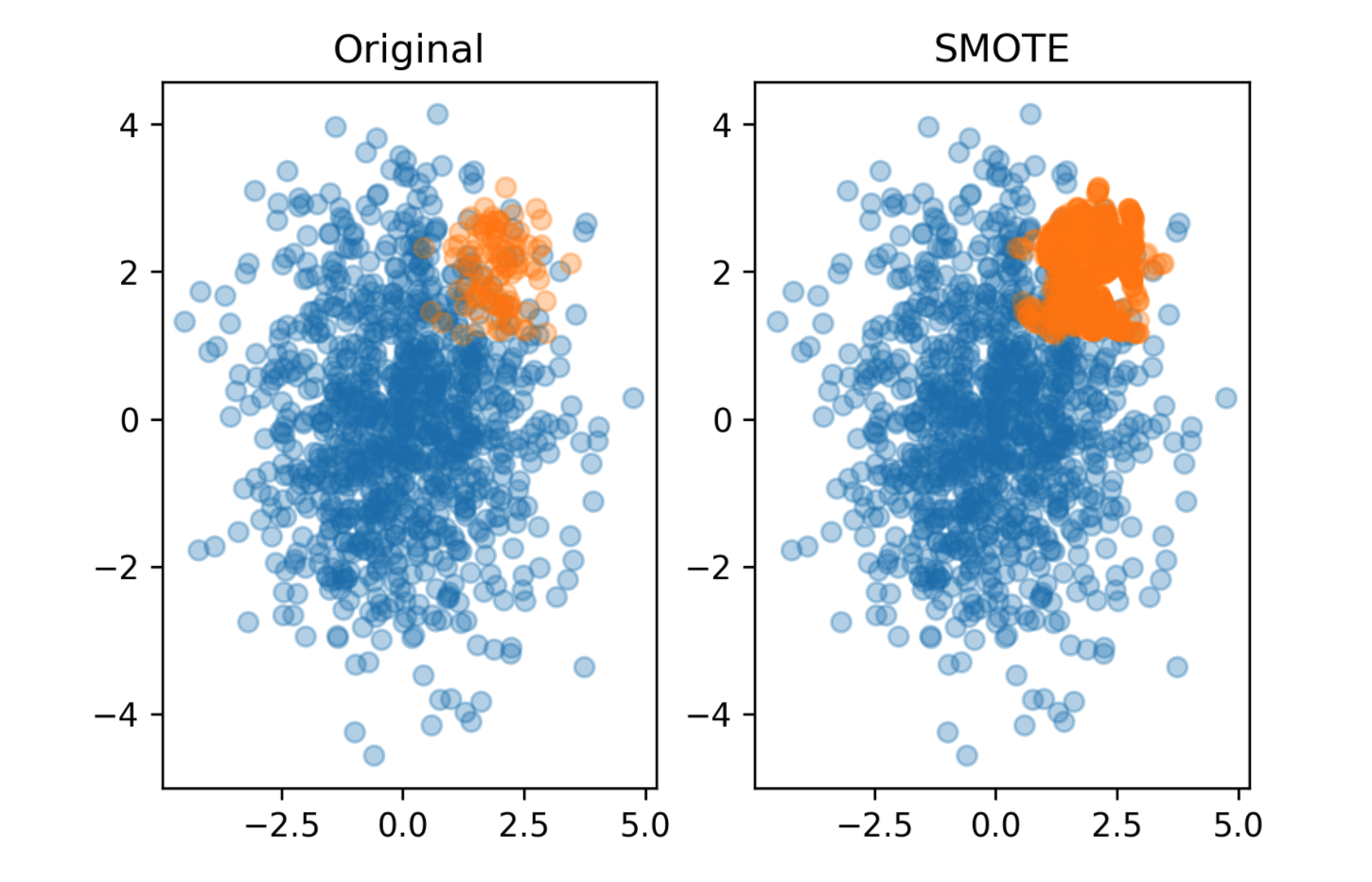
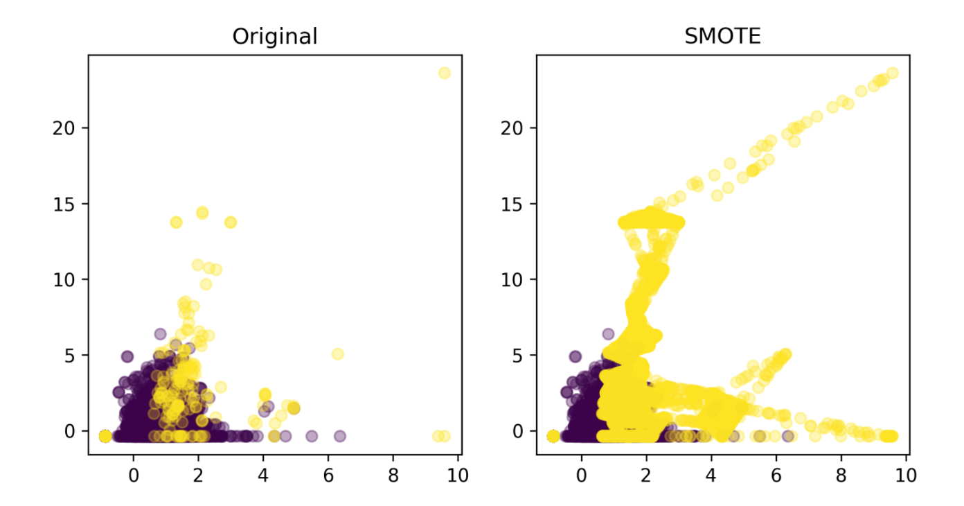
Synthetic Sample Generation

Synthetic Minority Oversampling Technique (SMOTE)

Adds synthetic interpolated data to smaller class
For each sample in minority class:
- Pick random neighbor from k neighbors.
- Pick point on line connecting the two uniformly
- Repeat.

from imblearn.over_sampling import SMOTE
smote_pipe = make_imb_pipeline(SMOTE(),
                               LogisticRegression(solver='lbfgs'))
scores = cross_val_score(smote_pipe, X_train, y_train,
                         cv=10, scoring='roc_auc')
print(f"{np.mean(scores):.3f}")

0.922

smote_pipe_rf = \
    make_imb_pipeline(SMOTE(),
                      RandomForestClassifier(n_estimators=100))
scores = cross_val_score(smote_pipe_rf,X_train,y_train,
                         cv=10, scoring='roc_auc')
print(f"{np.mean(scores):.3f}")

0.943

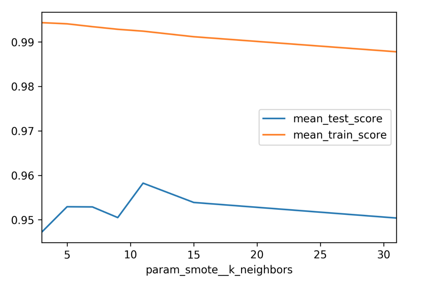
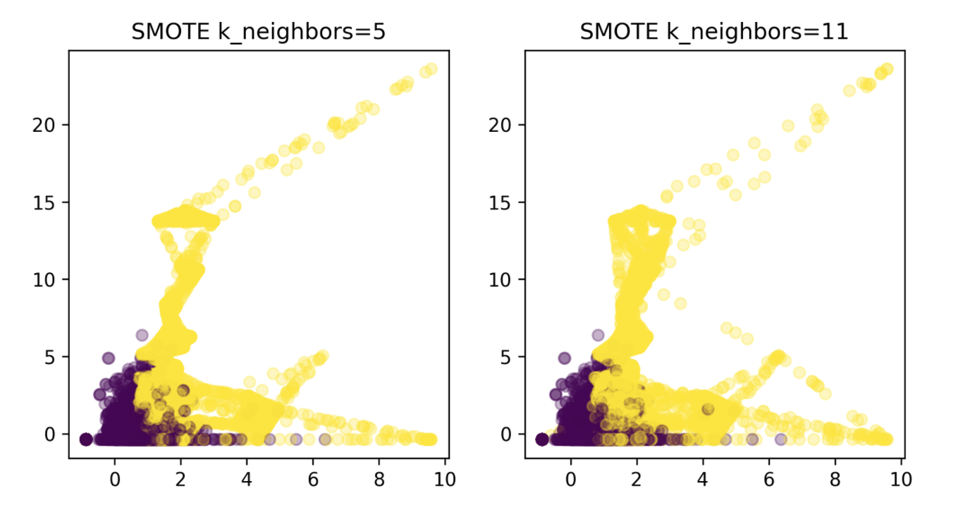
param_grid = {'smote__k_neighbors': [3, 5, 7, 9, 11, 15, 31]}
search = GridSearchCV(smote_pipe_rf, param_grid,
                      cv=10, scoring="roc_auc")
search.fit(X_train, y_train)
print(f"{search.score(X_test, y_test):.3f}")

0.959