Model Evaluation

09/14/2022

Robert Utterback (based on slides by Andreas Muller)

\( \renewcommand{\vec}[1]{\boldsymbol{#1}} \newcommand{\E}{\mathop{\boldsymbol{E}}} \newcommand{\var}{\boldsymbol{Var}} \newcommand{\norm}[1]{\lvert\lvert#1\rvert\rvert} \newcommand{\abs}[1]{\lvert#1\rvert} \newcommand{\ltwo}[1]{\norm{#1}_2} \newcommand{\lone}[1]{\norm{#1}_1} \newcommand{\sgn}[1]{\text{sign}\left( #1 \right)} \newcommand{\e}{\mathrm{e}} \newcommand{\minw}{\min_{w \in \mathbb{R}^p}} \newcommand{\sumn}{\sum_{i=1}^n} \newcommand{\logloss}{\log{(\exp{(-y_iw^T\vec{x}_i)} + 1)}} \)

Metrics for Binary Classification

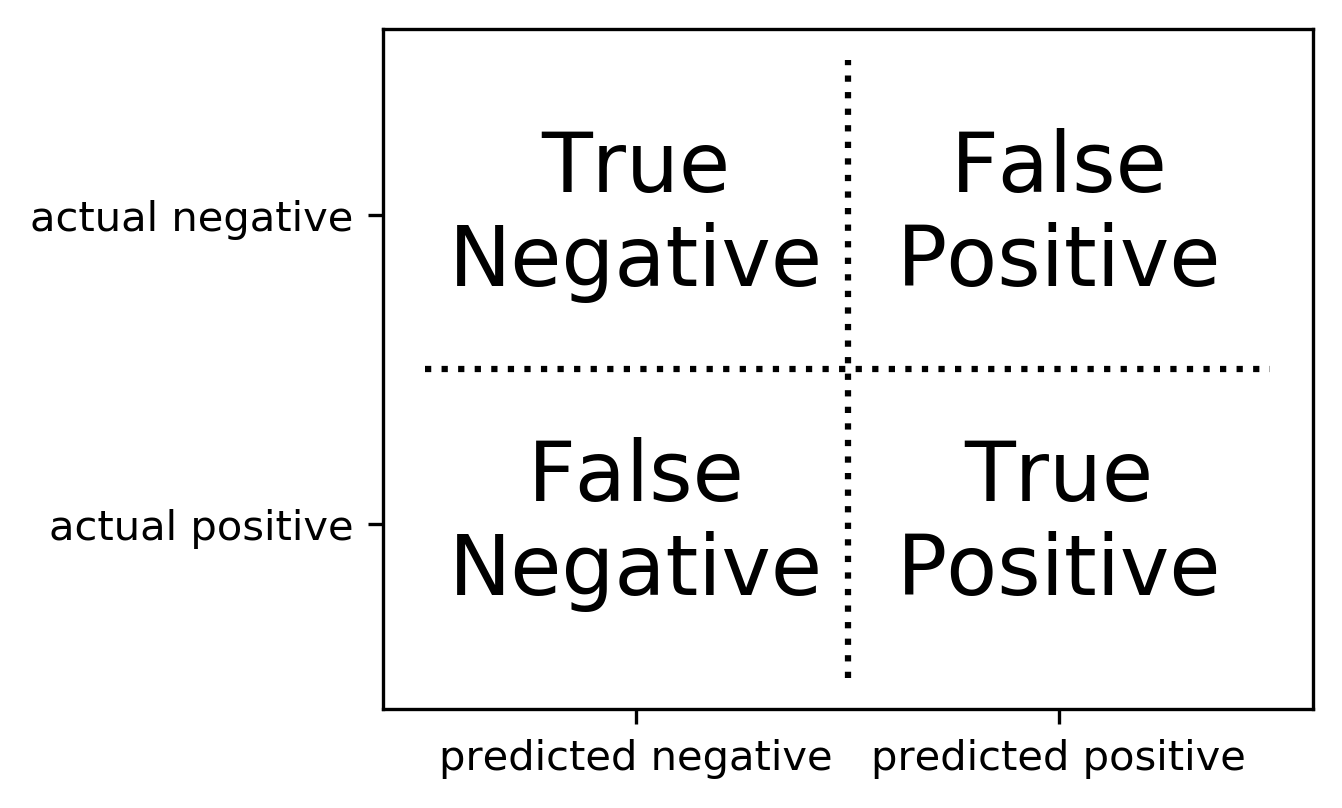
Confusion Matrix

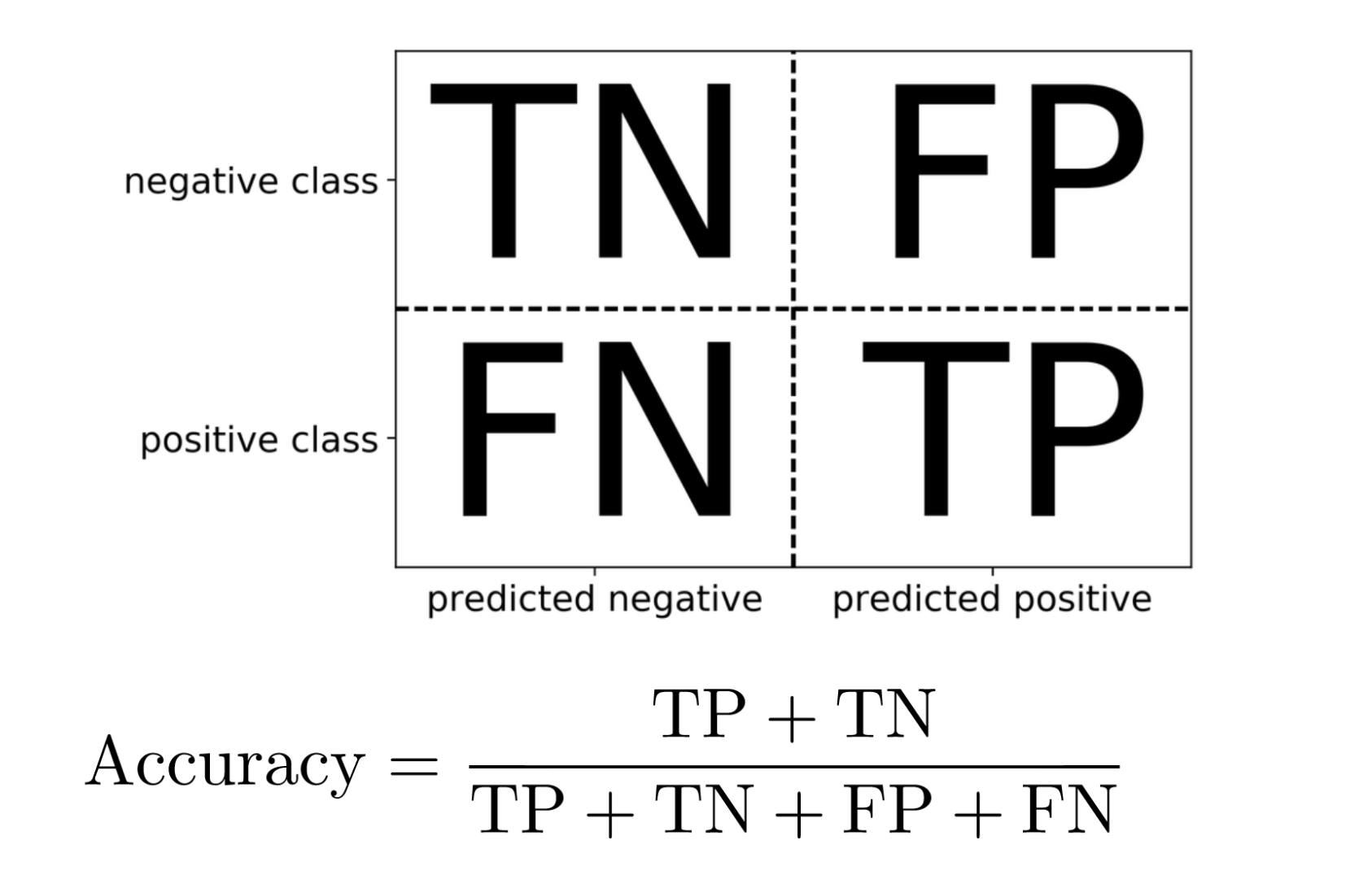
Positive vs. Negative

Pos. vs. Neg. is arbitrary!
(But often minority class = positive)

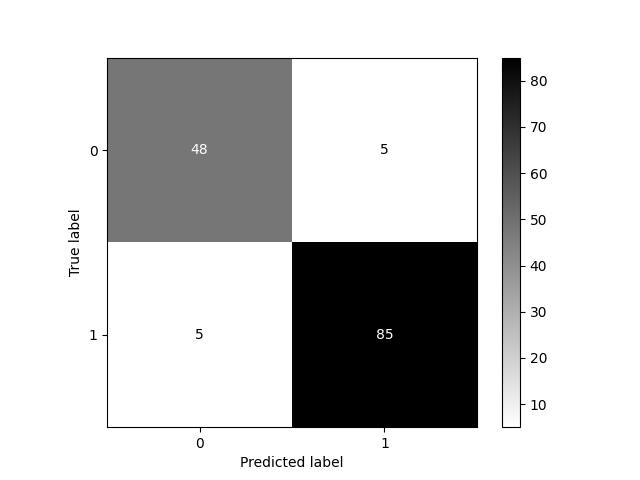
Confusion Matrix in Python

from sklearn.metrics import confusion_matrix, ConfusionMatrixDisplay
data = load_breast_cancer()
X_train, X_test, y_train, y_test = \
    train_test_split(data.data, data.target,
                     stratify=data.target, random_state=0)
lr = LogisticRegression().fit(X_train, y_train)
y_pred = lr.predict(X_test)
cm = confusion_matrix(y_test, y_pred)
print(cm)
print(f"{lr.score(X_test, y_test):.3f}")
ConfusionMatrixDisplay(confusion_matrix=cm).plot(cmap='gray_r')
plt.savefig('img/bc_conf_matrix.png')

[[48  5]
 [ 5 85]]
0.930

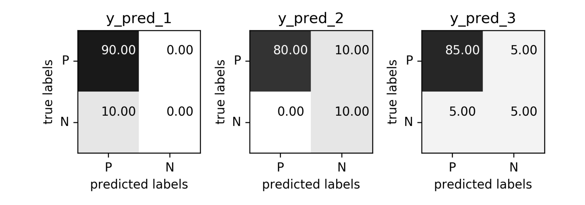
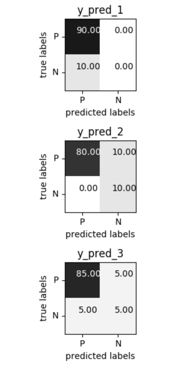
Problems with Accuracy

Data with 90% positives:

from sklearn.metrics import accuracy_score
for y_pred in [y_pred_1, y_pred_2, y_pred_3]:
    print(accuracy_score(y_true, y_pred))

0.9
0.9
0.9

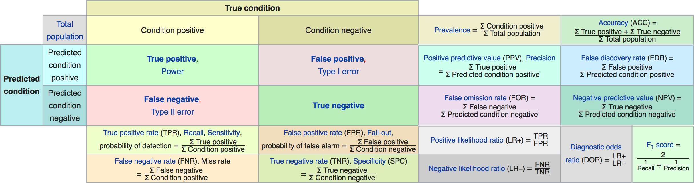
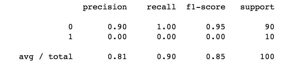
Precision, Recall, \(F_1\) -score

Precision, Positive Predictive Value (PPV):

\[ \frac{\text{TP}}{\text{TP}+\text{FP}} \]

Recall (sensitivity, coverage, true positive rate)

\[ \frac{\text{TP}}{\text{TP}+\text{FN}} \]

\(F_1\) -score (harmonic mean of precision and recall)

\[ 2 \frac{\text{precision} \cdot\text{recall}}{\text{precision}+\text{recall}} \]

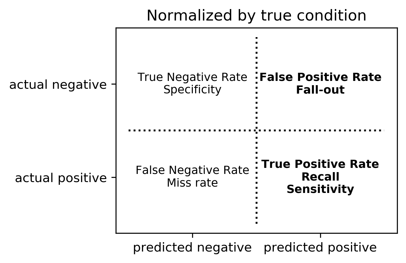
The Zoo

Normalizing the confusion matrix

confusion_matrix(y_true, y_pred)

confusion_matrix(y_true, y_pred, normalize='true')

confusion_matrix(y_true, y_pred, normalize='pred')

Averaging strategies

"macro", "weighted", "micro" (multi-label), "samples" (multi-label)

\[\text{macro }\frac{1}{\left|L\right|} \sum_{l \in L} R(y_l, \hat{y}_l)\] \[\text{weighted } \frac{1}{m} \sum_{l \in L} m_l R(y_l, \hat{y}_l)\]

w = recall_score(y_test, pred, average='weighted')
m = recall_score(y_test, pred, average='macro')
print(f"Weighted average: {w:.3f}")
print(f"Macro average: {m:.3f}")

Weighted average: 0.90
Macro average: 0.50

One common way to approach multiclass: look at averages over binary metrics
"micro" and "samples" have to do with multi-label prediction (each sample can have multiple labels)
We won't have time to talk about that in this class
Positive class is now label \(\ell\), negative is any other (like OVR)
So you're summing over all those recall values
Weighted weights by number of samples of that class, then divide by total # samples
This last I think is what classification report has at bottom of previous slide
Can also look at average precision instead of recall
weighted takes into account class sizes, so if you really care about the smaller classes you might want to choose macro
Let's say you have perfect recall for one class and 0 for the other.
Macro recall would be 0.5, but for weighted would be 0.9 if 90% of data is positive.
Choice comes down to: do you think each class should have equal weight or each sample should?
Macro: each class is same, Weighted: each sample is same

Balanced Accuracy

balanced_accuracy_score(y_t, y_p) == recall_score(y_t, y_p, average='macro')

\[ \text{balanced_accuracy} = \frac12 \left( \frac{TP}{TP+FN} + \frac{TN}{TN+FP} \right) \]

Always 0.5 for chance predictions
Equal to accuracy for balanced datasets

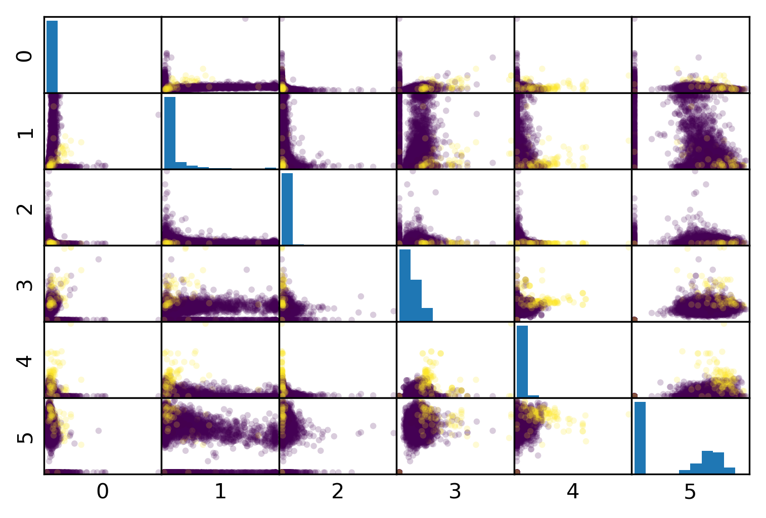
Mammography Data

from sklearn.datasets import fetch_openml
# mammography dataset https://www.openml.org/d/310
data = fetch_openml('mammography', as_frame=True)
X, y = data.data, data.target
print(X.shape)

(11183, 6)

print(y.value_counts())

-1    10923
1       260
Name: class, dtype: int64

# make y boolean -- allows sklearn to determine positive class more easily
X_train, X_test, y_train, y_test = train_test_split(X, y=='1', random_state=0)

Mammography Results

svc = make_pipeline(StandardScaler(),
                    SVC(C=100, gamma=0.1))
svc.fit(X_train, y_train)
print(f"{svc.score(X_test, y_test):.3f}")
print(classification_report(y_test, svc.predict(X_test)))

0.986
              precision    recall  f1-score   support

       False       0.99      1.00      0.99      2732
        True       0.81      0.53      0.64        64

    accuracy                           0.99      2796
   macro avg       0.90      0.76      0.82      2796
weighted avg       0.98      0.99      0.99      2796

rf = RandomForestClassifier()
rf.fit(X_train, y_train)
print(f"{rf.score(X_test, y_test):.3f}")
print(classification_report(y_test, rf.predict(X_test)))

0.988
              precision    recall  f1-score   support

       False       0.99      1.00      0.99      2732
        True       0.92      0.52      0.66        64

    accuracy                           0.99      2796
   macro avg       0.95      0.76      0.83      2796
weighted avg       0.99      0.99      0.99      2796

Goal setting!

What do I want? What do I care about?
Can I assign costs to the confusion matrix?
What guarantees do we want to give?

Changing Thresholds

data = load_breast_cancer()

X_train, X_test, y_train, y_test = \
    train_test_split(data.data, data.target,
                     stratify=data.target, random_state=0)

lr = LogisticRegression(solver='liblinear').fit(X_train, y_train)
y_pred = lr.predict(X_test)

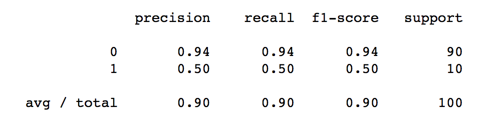
print(classification_report(y_test, y_pred))

              precision    recall  f1-score   support

           0       0.91      0.92      0.92        53
           1       0.96      0.94      0.95        90

    accuracy                           0.94       143
   macro avg       0.93      0.93      0.93       143
weighted avg       0.94      0.94      0.94       143

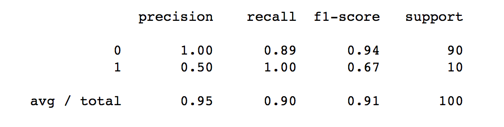
y_pred = lr.predict_proba(X_test)[:, 1] > .85

print(classification_report(y_test, y_pred))

              precision    recall  f1-score   support

           0       0.85      1.00      0.92        53
           1       1.00      0.90      0.95        90

    accuracy                           0.94       143
   macro avg       0.93      0.95      0.93       143
weighted avg       0.95      0.94      0.94       143

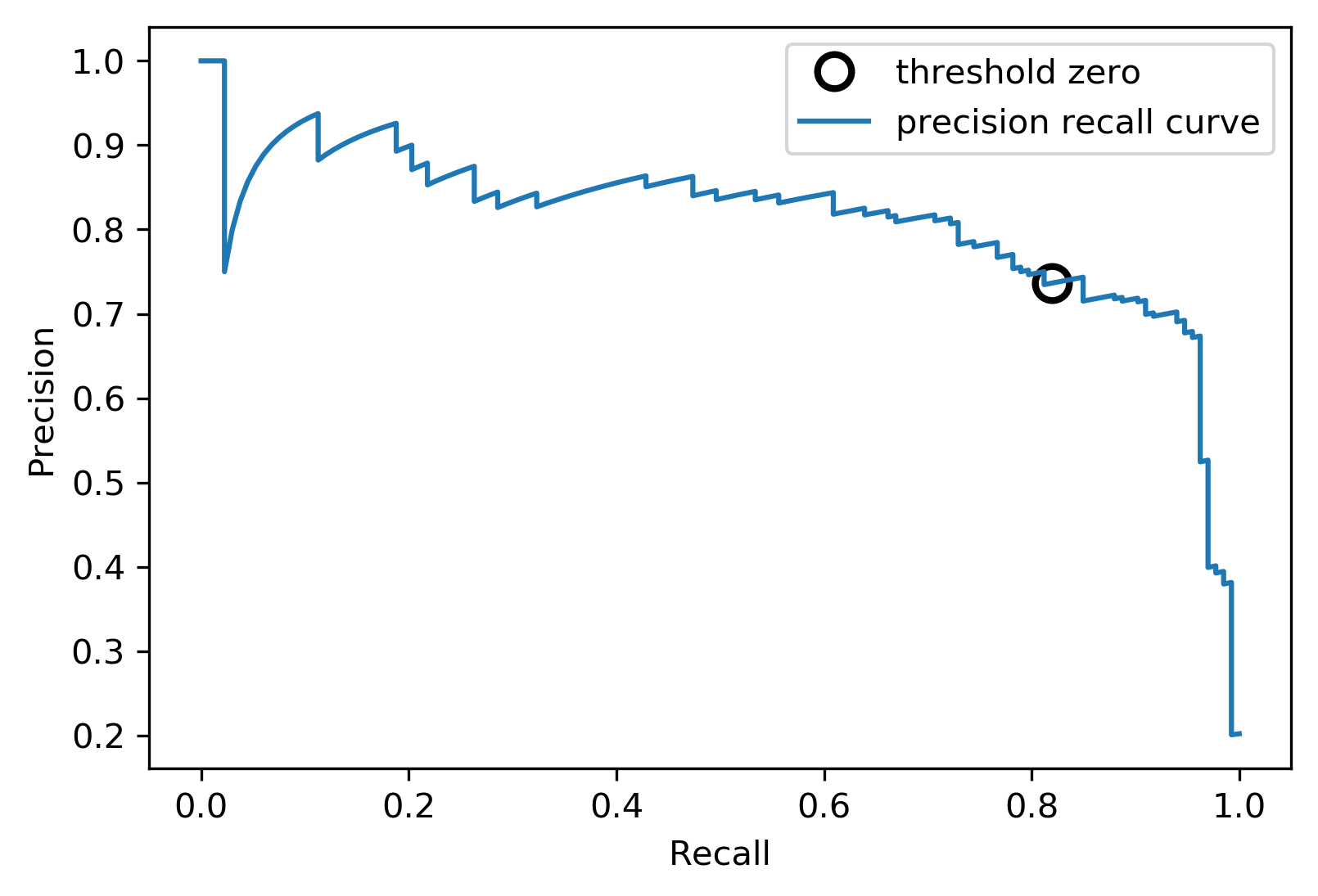
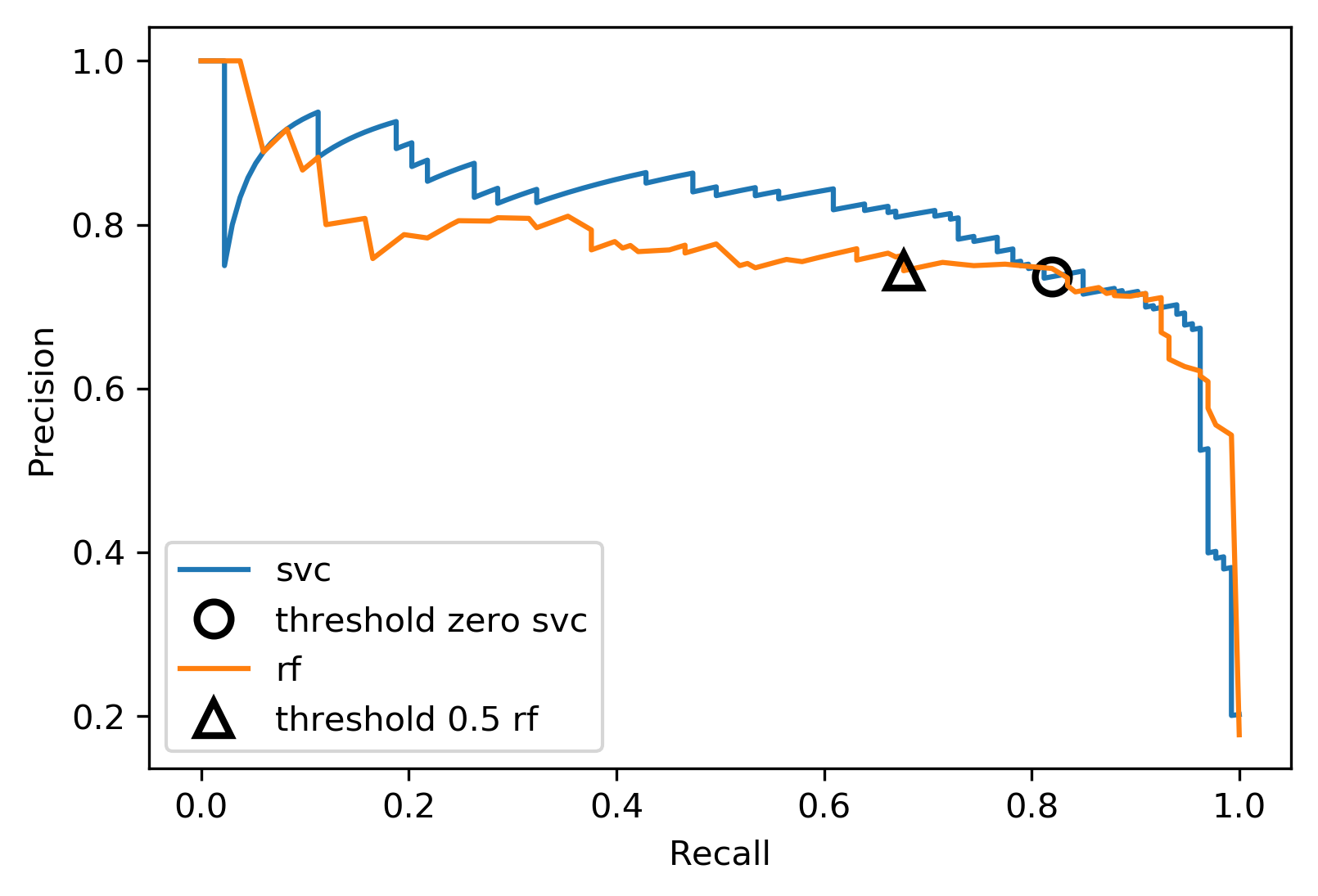
Precision-Recall curve

X, y = make_blobs(n_samples=(2500, 500), cluster_std=[7.0, 2],
                  random_state=22)

X_train, X_test, y_train, y_test = train_test_split(X, y)

svc = SVC(gamma=.05).fit(X_train, y_train)

precision, recall, thresholds = precision_recall_curve(
    y_test, svc.decision_function(X_test))

Precision-Recall curve

Comparing RF and SVC

Average Precision

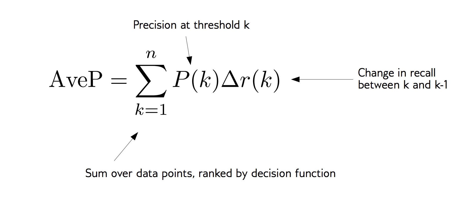
\(F_1\) vs Average Precision

from sklearn.metrics import f1_score
rf_score = f1_score(y_test, rf.predict(X_test))
print(f"f1_score of random forest: {rf_score:.3f}")
svc_score = f1_score(y_test, svc.predict(X_test))
print(f"f1_score of svc: {svc_score:.3f}")

f1_score of random forest: 0.683
f1_score of svc: 0.800

from sklearn.metrics import average_precision_score
ap_rf = average_precision_score(
    y_test,rf.predict_proba(X_test)[:, 1])
ap_svc = average_precision_score(
    y_test, svc.decision_function(X_test))
print(f"Average precision of random forest: {ap_rf:.3f}")
print(f"Average precision of svc: {ap_svc:.3f}")

Average precision of random forest: 0.674
Average precision of svc: 0.791

ROC Curve

\[ \text{FPR} = \frac{\text{FP}}{\text{FP}+\text{TN}}\]

\[ \text{TPR} = \frac{\text{TP}}{\text{TP}+\text{FN}} = \text{recall}\]

ROC Curve

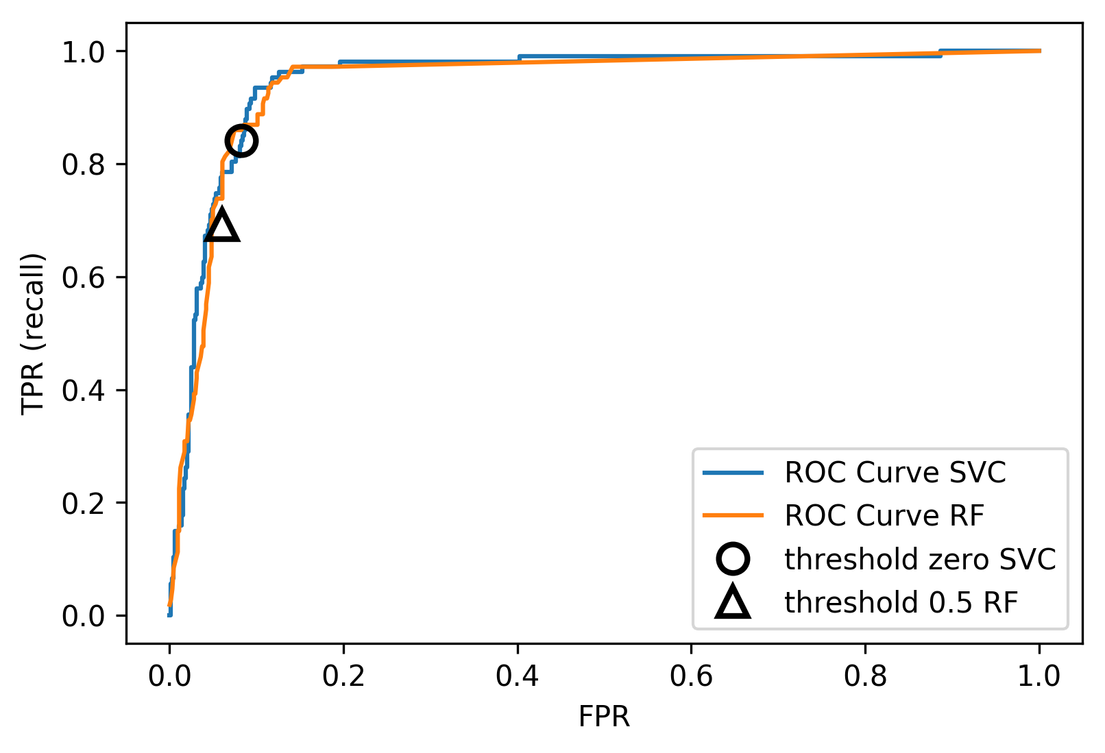
ROC AUC

Area under ROC Curve
Always .5 for random/constant prediction

from sklearn.metrics import roc_auc_score
rf_auc = roc_auc_score(y_test, rf.predict_proba(X_test)[:,1],
                       multi_class='ovr')
svc_auc = roc_auc_score(y_test, svc.decision_function(X_test))
print(f"AUC for random forest: {rf_auc:.3f}")
print(f"AUC for SVC: {svc_auc:.3f}")

AUC for random forest: 0.944
AUC for SVC: 0.958

Summary of metrics for binary classification

Threshold-based:

accuracy
precision, recall, f1

Ranking:

average precision
ROC AUC

Multiclass Classification

Hack: Reduction to Binary Classification

One vs. Rest
One vs. One

One vs. Rest (OVR)

For 4 classes:
- A vs. {B,C,D}, B vs. {A,C,D}, C vs. {A,B,D}, D vs. {A,B,C}
In general:
- \(c\) binary classifiers, each on all data points

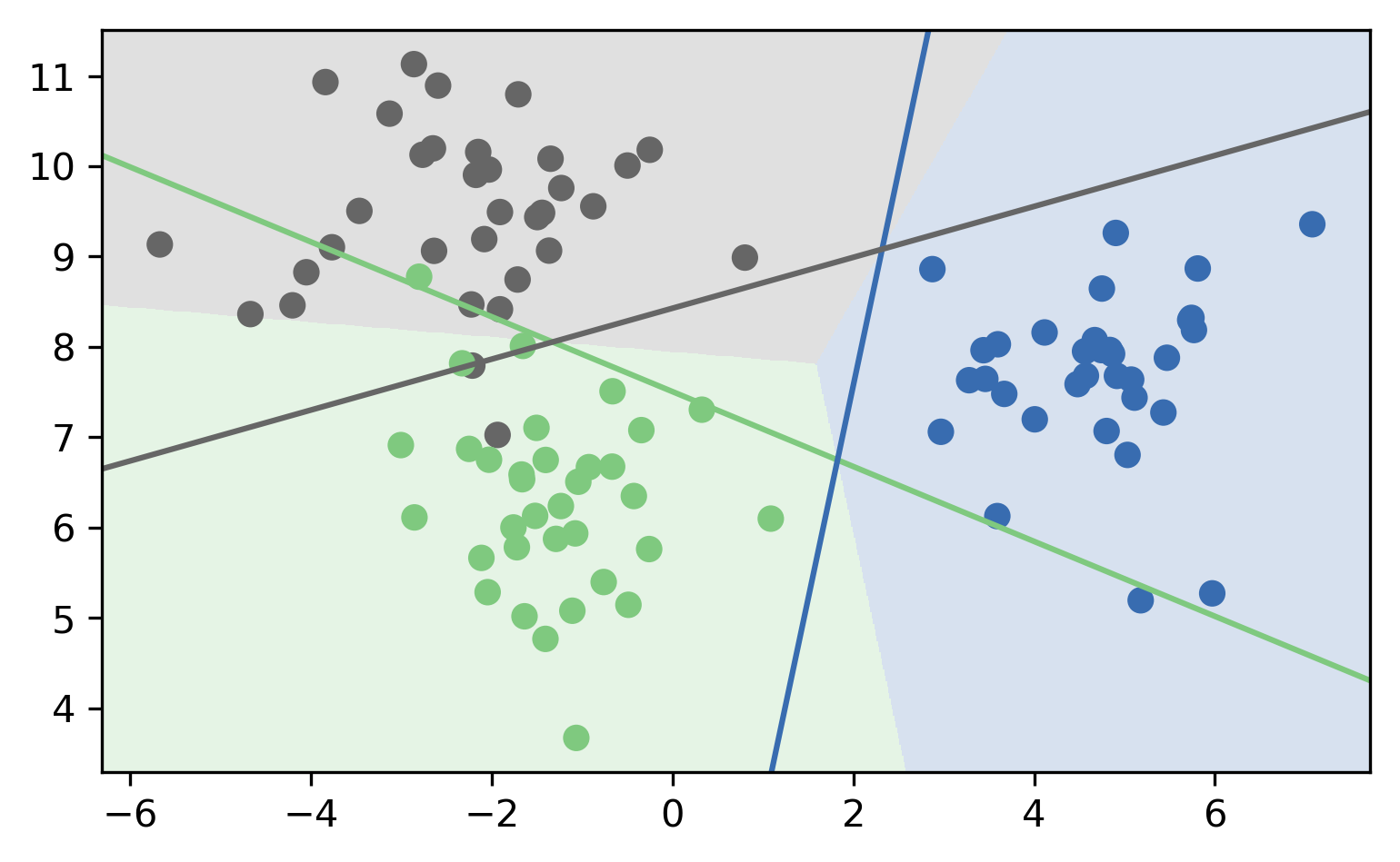
Prediction with OVR

Pick class with highest score: \[ \hat{y} = \text{argmax}_{i \in Y} \vec{w}_i^T \vec{x} \]
Unclear why it works, but works well.

OVR Prediction

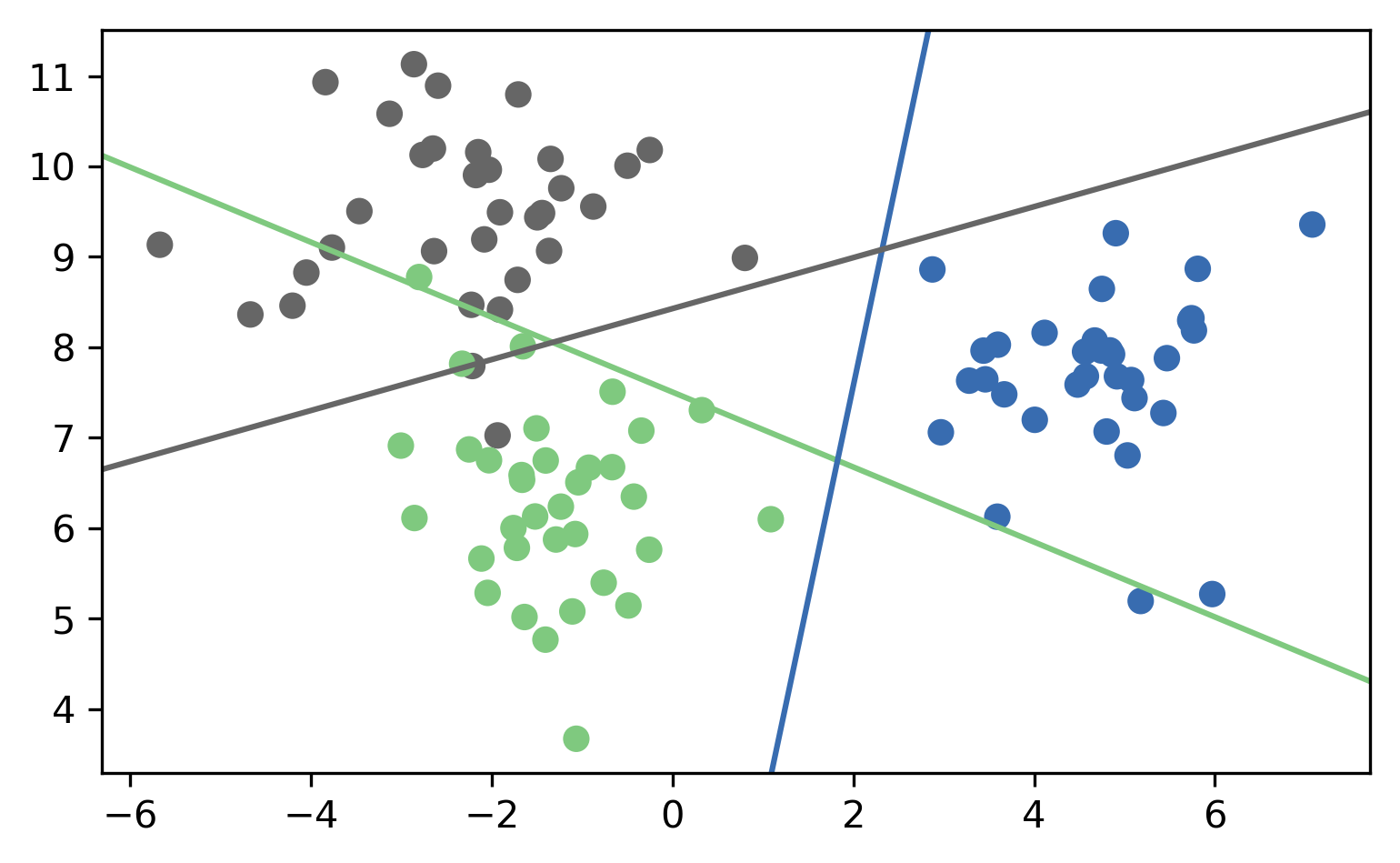
OVR Prediction Boundaries

One Vs. One (OVO)

A vs. B, A vs. C, A vs. D, B vs. C, B vs. D, C vs. D
\({c\choose{2}} = \frac{c(c-1)}{2}\) binary classifiers
- each trained on a fraction of the data
Vote for highest positives
- Classify on all classifiers
- Count how often each class was predicted
- Return most commonly predicted class
Works well, but again a heuristic

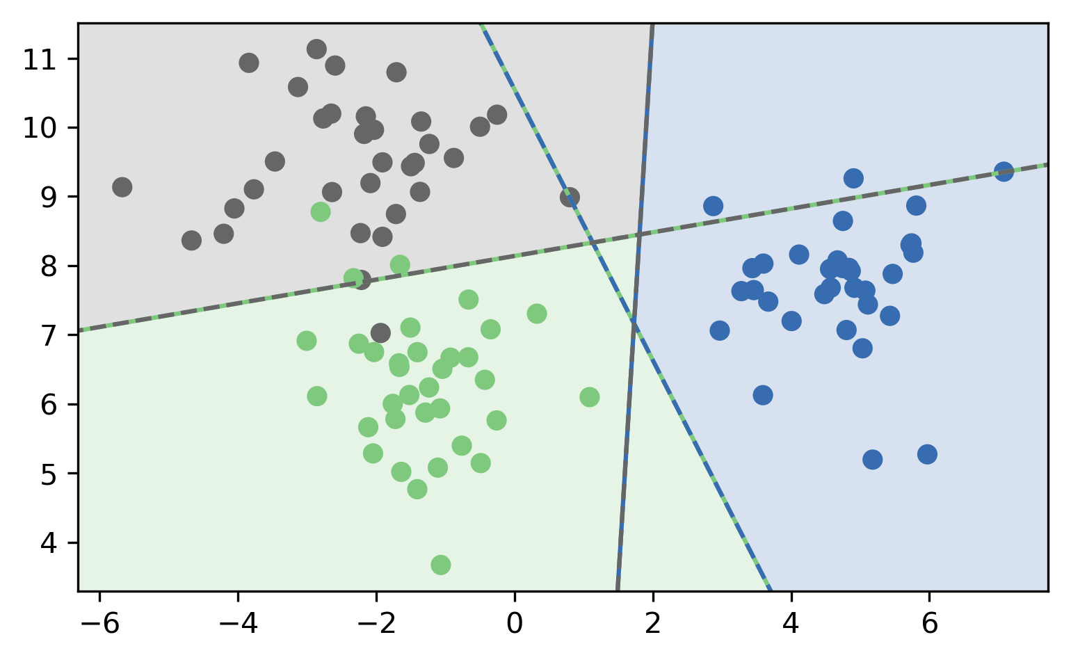
OVO Prediction

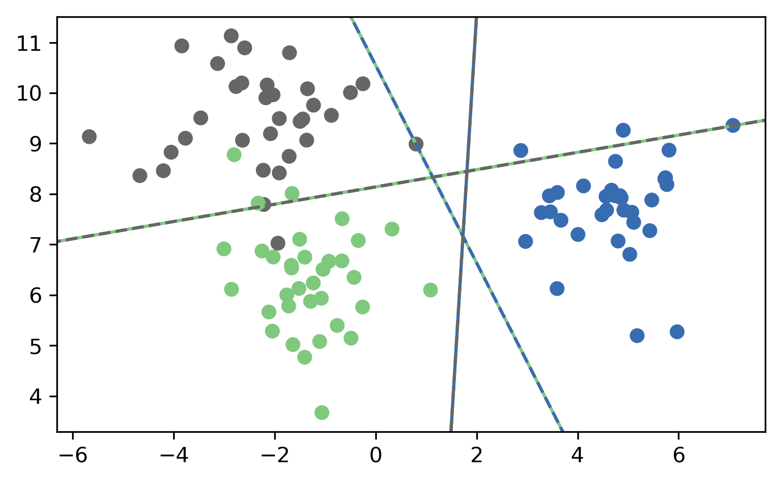
OVO Prediction Boundaries

Looking at the predictions made by the one vs one classifier the correspondence to the binary decision boundaries is a bit more clear than for the one vs rest heuristic, because it only takes the actual boundaries into account, not the length of the normal vectors. That makes it easier to visualize the geometry, but it's also a bit of a downside of the method because it means it discards any notion of uncertainty that was present in the binary classifiers. The decision boundary for each class is given by the two lines that this class is involved in. So the grey class is bounded by the green and grey line and the blue and grey line.

There is a triangle in the center in which there is one vote for each of the classes. In this implemenatation the tie is broken to just always predict the first class, which is the green one. That might not be the best tie breaking strategy, but this is a relatively rare case, in particular if there's more than three classes.

OVR and OVO are general heuristics not restricted to linear models. They can be used whenever a binary model for classification needs to be extended to the multi-class case. For logistic regression, there is actually a natural extension of the formulation, and we don't have to resort to these hacks.

OVR-OVO Comparison

OVR:

\(c\) classifiers
trained on imbalanced datasets of original size
Retains some uncertainty estimates

OVO:

\(c(c-1)/2\) classifiers
trained on balanced subsets
No uncertainty propagated

Multinomial Logistic Regression

\[ p(y=i | x) = \frac{\e^{w_{i}^T \vec{x}}}{\sum_j \e^{w_{j}^T \vec{x}}} \] \[ \minw \sum_{i=1}^c \log(p(y=y_i | x_i)) \] \[ \hat{y} = \text{argmax}_{i \in Y} w_i \vec{x} \]

Same prediction rule as OVR.

In scikit-learn

OVO: Only SVC
OVR: default for all linear models except LogisticRegression
clf.decision_function \(=w^T x\)
clf.predict_proba gives probabilities for each class
SVC(probability=True) not great

Multiclass in Practice

iris = load_iris()
X,y = iris.data, iris.target
print(X.shape)
print(np.bincount(y))

logreg = LogisticRegression(multi_class="multinomial",
                            random_state=0,
                            solver="lbfgs").fit(X,y)
linearsvm = LinearSVC().fit(X,y)
print(logreg.coef_.shape)
print(linearsvm.coef_.shape)

(150, 4)
[50 50 50]
(3, 4)
(3, 4)

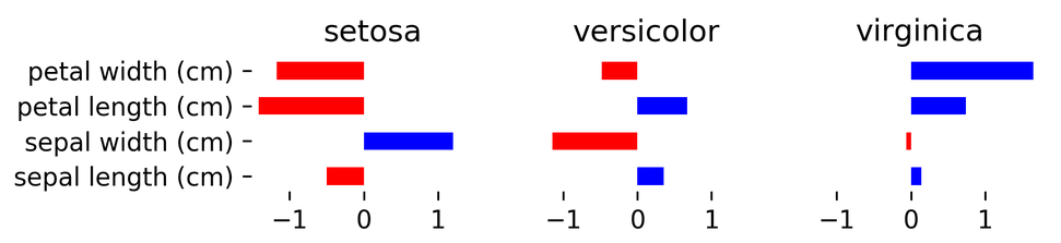
logreg.coef_

Multi-class classification

Confusion Matrix

from sklearn.datasets import load_digits
from sklearn.metrics import accuracy_score

digits = load_digits()
# data is between 0 and 16
X_train, X_test, y_train, y_test = \
    train_test_split(digits.data / 16.,
                     digits.target, random_state=0)
lr = LogisticRegression().fit(X_train, y_train)
pred = lr.predict(X_test)
print(f"Accuracy: {accuracy_score(y_test, pred):.3f}")
print(confusion_matrix(y_test, pred))

Accuracy: 0.962
[[37  0  0  0  0  0  0  0  0  0]
 [ 0 40  0  0  0  0  1  0  1  1]
 [ 0  0 44  0  0  0  0  0  0  0]
 [ 0  0  0 43  0  0  0  0  1  1]
 [ 0  0  0  0 37  0  0  1  0  0]
 [ 0  0  0  0  0 46  0  0  0  2]
 [ 0  1  0  0  0  0 51  0  0  0]
 [ 0  0  0  0  2  0  0 46  0  0]
 [ 0  3  1  0  0  1  0  0 43  0]
 [ 0  0  0  0  0  1  0  0  0 46]]

print(classification_report(y_test, pred))

              precision    recall  f1-score   support

           0       1.00      1.00      1.00        37
           1       0.91      0.93      0.92        43
           2       0.98      1.00      0.99        44
           3       1.00      0.96      0.98        45
           4       0.95      0.97      0.96        38
           5       0.96      0.96      0.96        48
           6       0.98      0.98      0.98        52
           7       0.98      0.96      0.97        48
           8       0.96      0.90      0.92        48
           9       0.92      0.98      0.95        47

    accuracy                           0.96       450
   macro avg       0.96      0.96      0.96       450
weighted avg       0.96      0.96      0.96       450

Multi-class ROC AUC

Hand & Till, 2001, one vs one

\[ \frac{1}{c(c-1)}\sum_{j=1}^{c}\sum_{k \neq j}^{c} AUC(j,k)\]

Provost & Domingo, 2000, one vs rest

\[ \frac{1}{c}\sum_{j=1}^{c}p(j) AUC(j,\text{rest}_j)\]

Summary of metrics for multiclass classification

Threshold-based:

accuracy
precision, recall, f1 (macro average, weighted)

Ranking:

OVR ROC AUC
OVO ROC AUC

Picking Metrics

Picking metrics

Accuracy rarely what you want
Problems are rarely balanced
Find the right criterion for the task
OR pick one arbitrarily, but at least think about it
Emphasis on recall or precision?
Which classes are the important ones?

Using metrics in cross-validation

X, y = make_blobs(n_samples=(2500, 500), cluster_std=[7.0, 2],
                  random_state=22)
# default scoring for classification is accuracy
scores_default = cross_val_score(SVC(gamma='auto'), X, y, cv=3)

# providing scoring="accuracy" doesn't change the results
explicit_accuracy =  cross_val_score(SVC(gamma='auto'), X, y,
                                     scoring="accuracy", cv=3)
# using ROC AUC
roc_auc =  cross_val_score(SVC(gamma='auto'), X, y, scoring="roc_auc", cv=3)
print(f"Default scoring: {scores_default}")
print(f"Explicit accuracy scoring: {explicit_accuracy}")
print(f"AUC scoring: {roc_auc}")

Default scoring: [0.92  0.904 0.913]
Explicit accuracy scoring: [0.92  0.904 0.913]
AUC scoring: [0.93  0.885 0.923]

Built-in scoring

from sklearn.metrics import get_scorer_names
print("\n".join(sorted(get_scorer_names())))

accuracy
adjusted_mutual_info_score
adjusted_rand_score
average_precision
completeness_score
explained_variance
f1
f1_macro
f1_micro
f1_samples
f1_weighted
fowlkes_mallows_score
homogeneity_score

log_loss
mean_absolute_error
mean_squared_error
median_absolute_error
mutual_info_score
neg_log_loss
neg_mean_absolute_error
neg_mean_squared_error
neg_mean_squared_log_error
neg_median_absolute_error
normalized_mutual_info_score
precision
precision_macro

precision_micro
precision_samples
precision_weighted
r2
recall
recall_macro
recall_micro
recall_samples
recall_weighted
roc_auc
v_measure_score

Providing you your own callable

Takes estimator, X, y
Returns score – higher is better (always!)

def accuracy_scoring(est, X, y):
      return (est.predict(X) == y).mean()

You can access the model!

from sklearn.model_selection import GridSearchCV

param_grid = {'C': np.logspace(-3, 2, 6),
 'gamma': np.logspace(-3, 2, 6) / X_train.shape[0]}
grid = GridSearchCV(SVC(), param_grid=param_grid, cv=10)
grid.fit(X_train, y_train)
print(grid.best_params_)
print(grid.score(X_test, y_test))
print(len(grid.best_estimator_.support_))

{'C': 10.0, 'gamma': 0.07423904974016332}
0.9911111111111112
498

def few_support_vectors(est, X, y):
    acc = est.score(X, y)
    frac_sv = len(est.support_) / np.max(est.support_)
    # Just made this up, don't use
    return acc / frac_sv

param_grid = {'C': np.logspace(-3, 2, 6),
 'gamma': np.logspace(-3, 2, 6) / X_train.shape[0]}
grid = GridSearchCV(SVC(), param_grid=param_grid, cv=10,
                    scoring=few_support_vectors)
grid.fit(X_train, y_train)
print(grid.best_params_)
print((grid.predict(X_test) == y_test).mean())
print(len(grid.best_estimator_.support_))

{'C': 100.0, 'gamma': 0.007423904974016332}
0.9777777777777777
405

Metrics for Regression

Built-in Standard Metrics

\(R^2\): easy to understand scale
MSE: easy to relate to input
Mean/Median absolute error: more robust
When using "scoring" use neg_mean_squared_error etc.

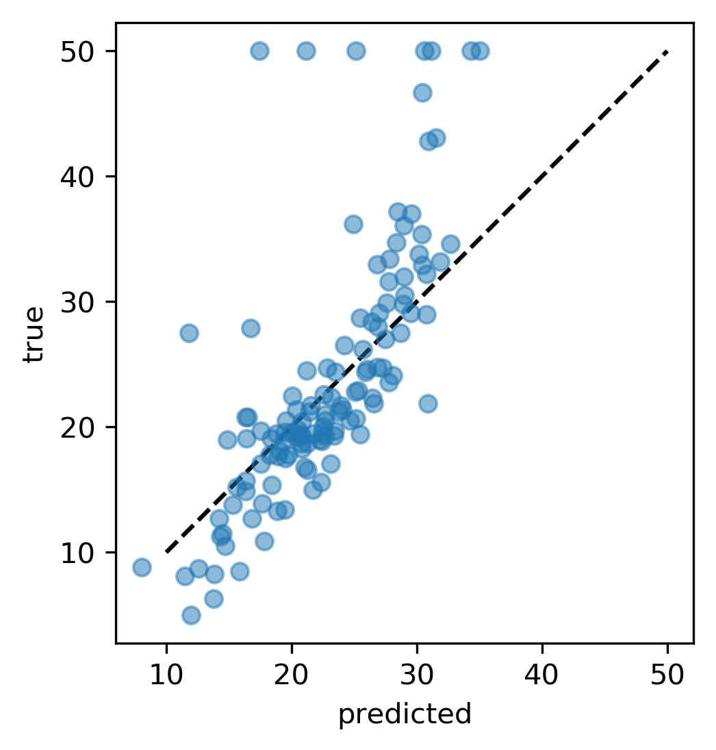
Prediction Plots

from sklearn.linear_model import Ridge
from sklearn.datasets import load_boston
boston = load_boston()
X_train, X_test, y_train, y_test = \
    train_test_split(boston.data, boston.target)
ridge = Ridge(normalize=True)
ridge.fit(X_train, y_train)
pred = ridge.predict(X_test)
plt.plot(pred, y_test, 'o')

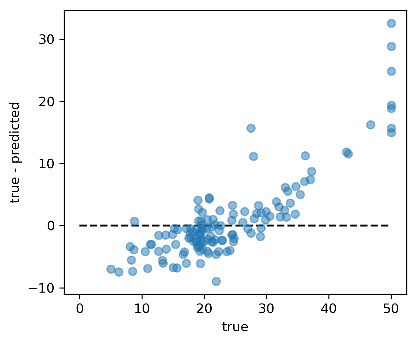
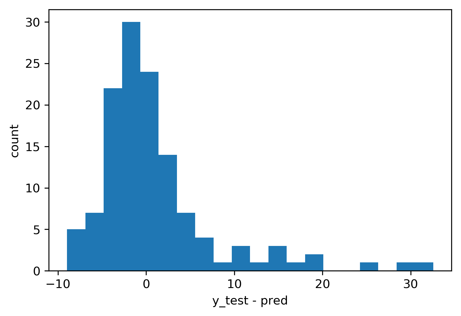
Residual Plots

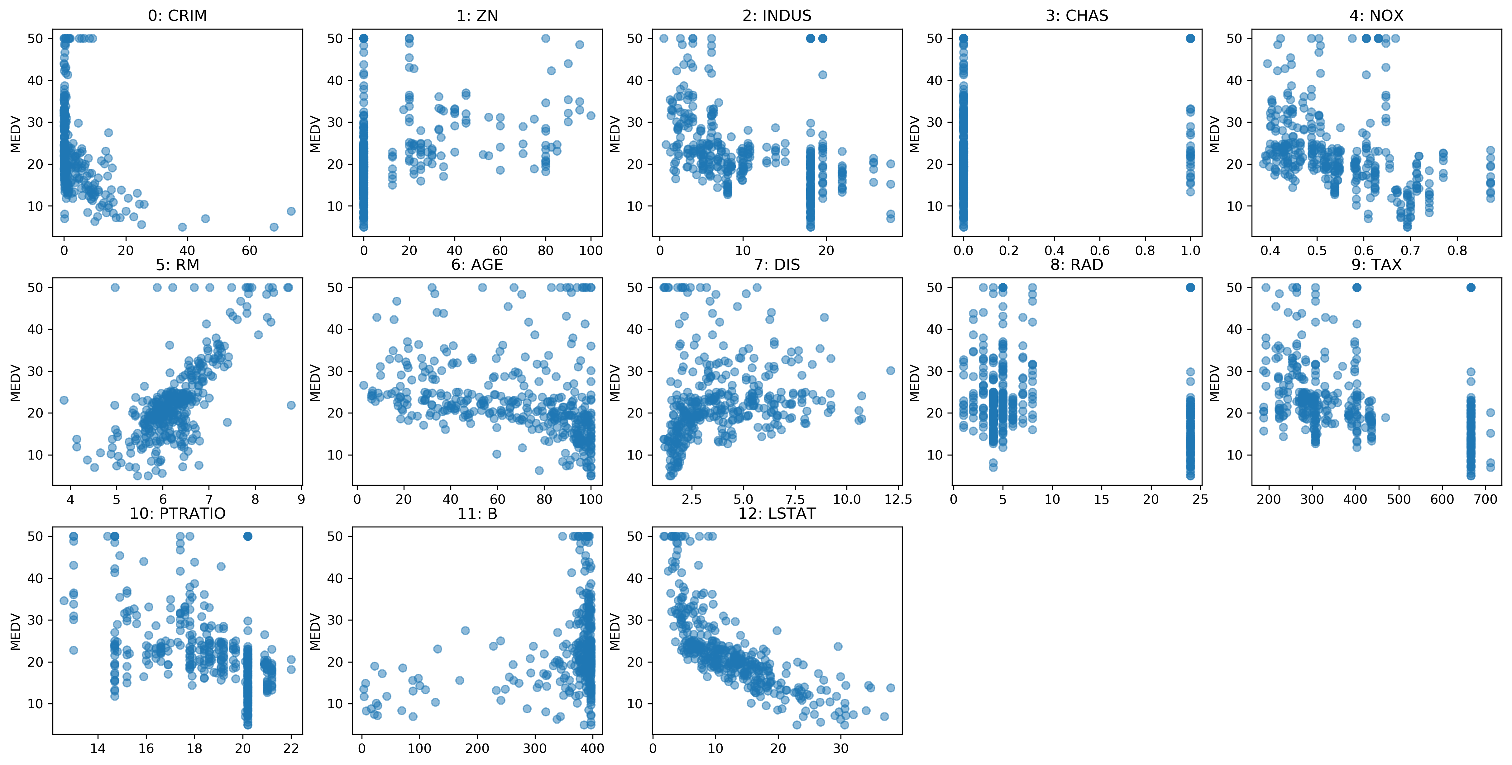
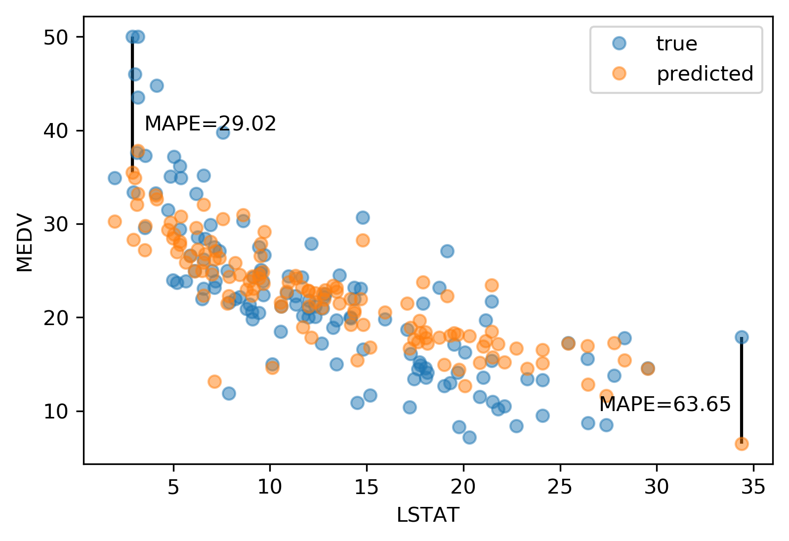
Target vs Feature

Residual vs Feature

Absolute vs Relative: MAPE

Mean Absolute Percentage Error

\[ \text{MAPE} = \frac{100}{m} \sum_{i=1}^{m}\left|\frac{y-\hat{y}}{y}\right|\]

Another metric: Mean Absolute Percentage Error
Captures the percentage error
It's got a residual, clearly taking a mean, and taking absolute value b/c that's all we care about
Interesting thing is the division of the residual by the true value (e.g., housing price)
If a data point is large, we don't care as much about prediction error, since the value is large anyway
For small values we care more
Which is intuitive: if a house costs 25 million, it doesn't matter that much if you predict a million off
But if a house is 50,000, you better not be off by a million!
Notice the two pairs on the plot, the absolute error between them vs. MAPE
Often used in forecasting (predicting future, like stock prices)
Careful, it might not be intuitive
If anything is zero, well it's not defined
If something is close to zero, you basically have to be perfect or else the percentage error will be very large

Over vs under

Overprediction and underprediction can have different cost.
Try to create cost-matrix: how much does overprediction and underprediction cost?
Is it linear?