Preprocessing

09/09/2022

Robert Utterback (based on slides by Andreas Muller)

Preprocessing

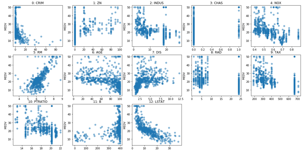
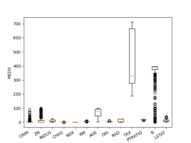
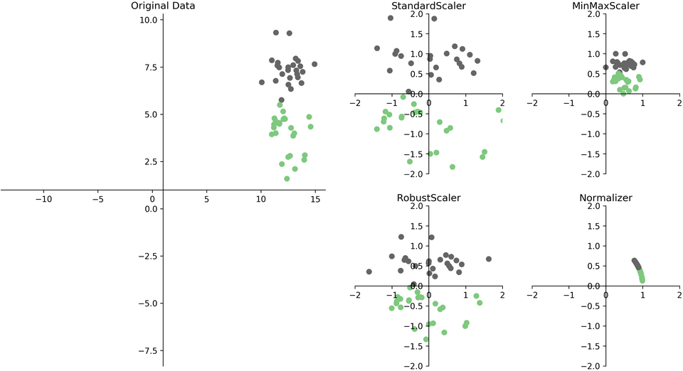
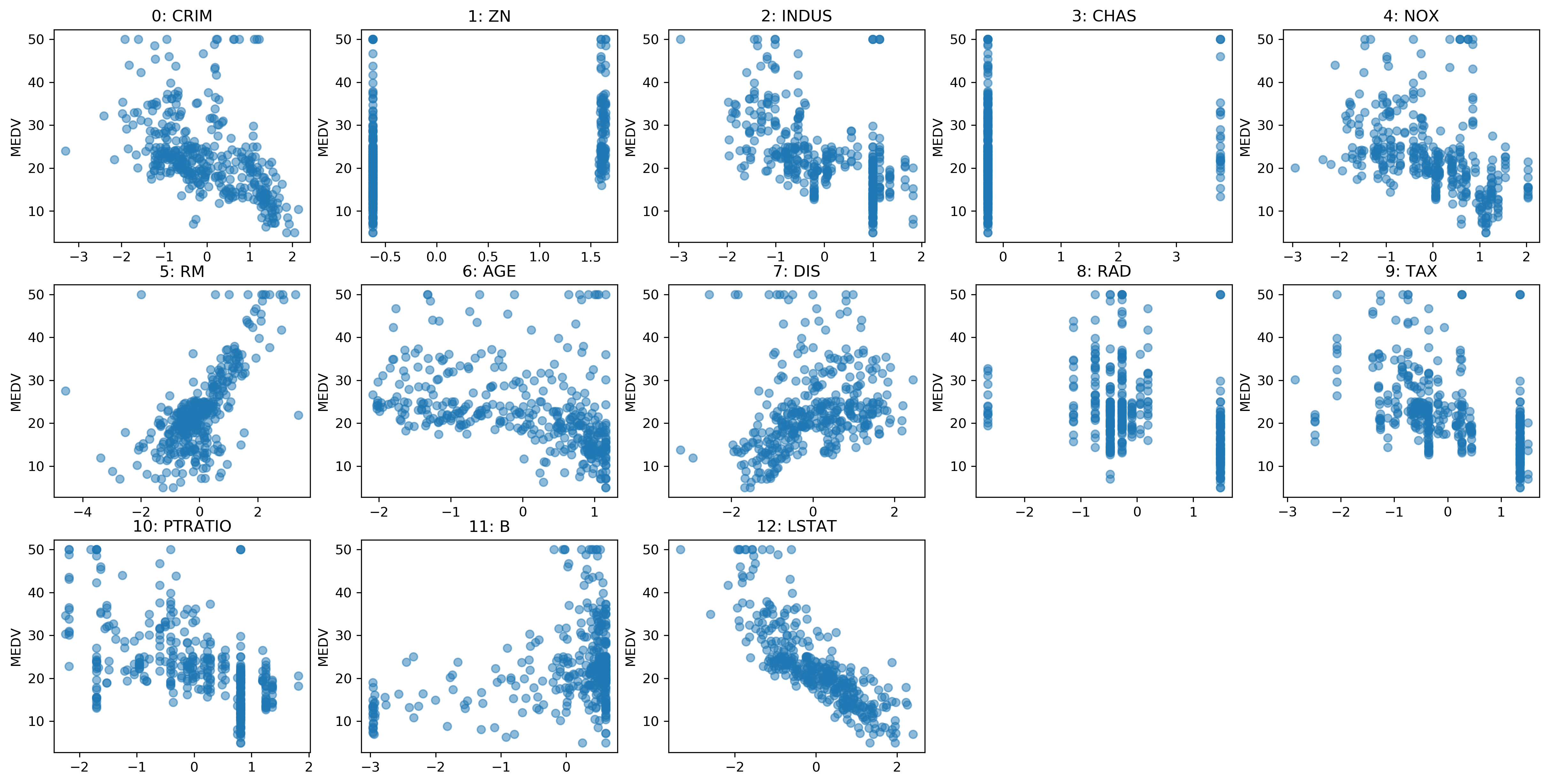
Scaling

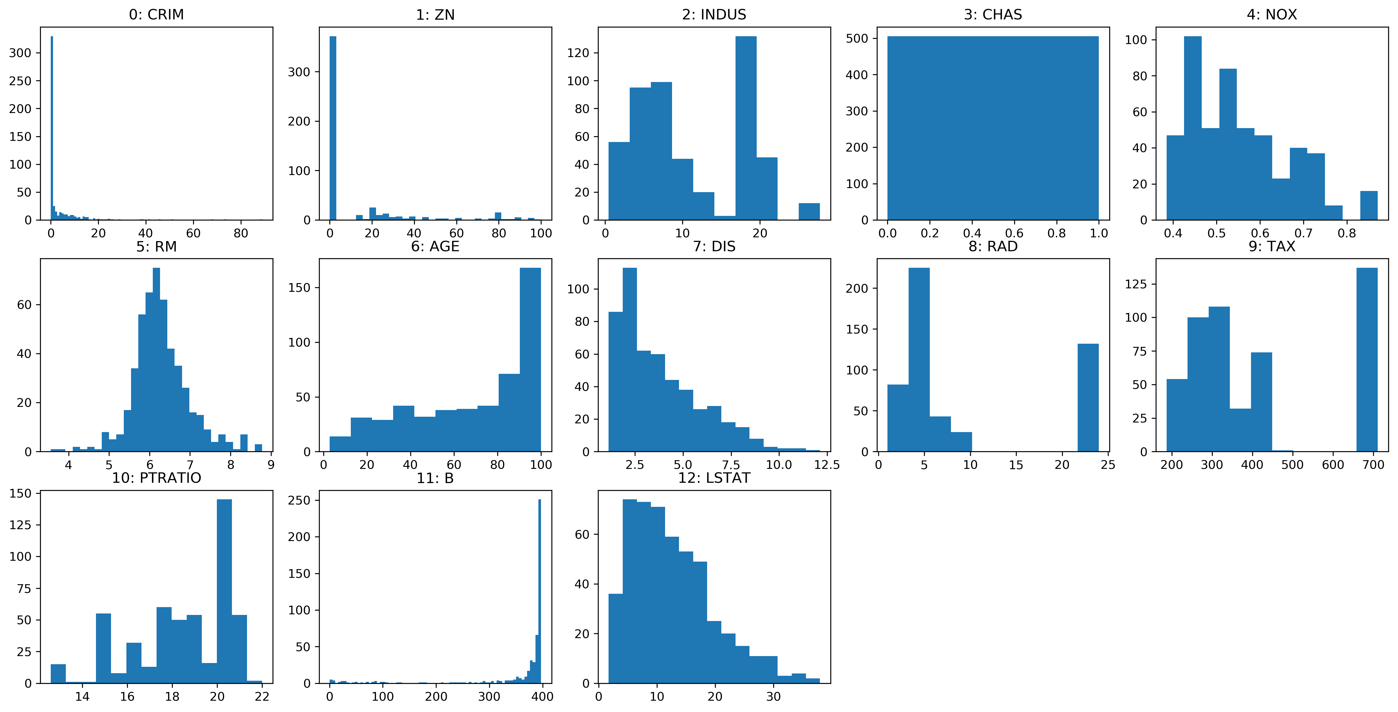
plt.figure()
plt.boxplot(X)
plt.xticks(np.arange(1, X.shape[1] + 1), features,
		   rotation=30, ha="right")
plt.ylabel("MEDV")

Scaling and Distances

Ways to Scale Data

Sparse Data

Data with many zeros — only store non-zero entries
Subtracting anything will make data "dense" — often can't fit in memory
Only scale, don't center (MaxAbsScaler)

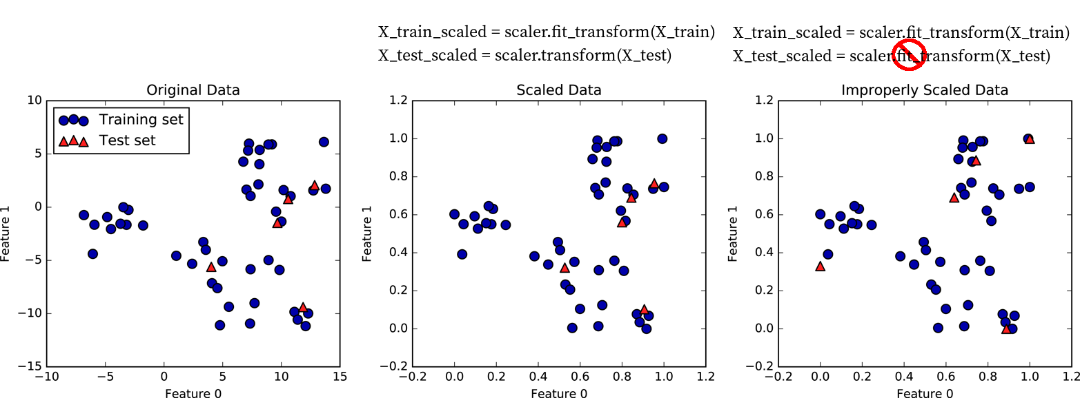
Standard Scaler Example

from sklearn.preprocessing import StandardScaler
X_train, X_test, y_train, y_test = \
	train_test_split(X, y, random_state=0)
scaler = StandardScaler()
scaler.fit(X_train)
X_train_scaled = scaler.transform(X_train)

ridge = Ridge().fit(X_train_scaled, y_train)
X_test_scaled = scaler.transform(X_test)
print("{:.2f}".format(ridge.score(X_test_scaled, y_test)))

0.63

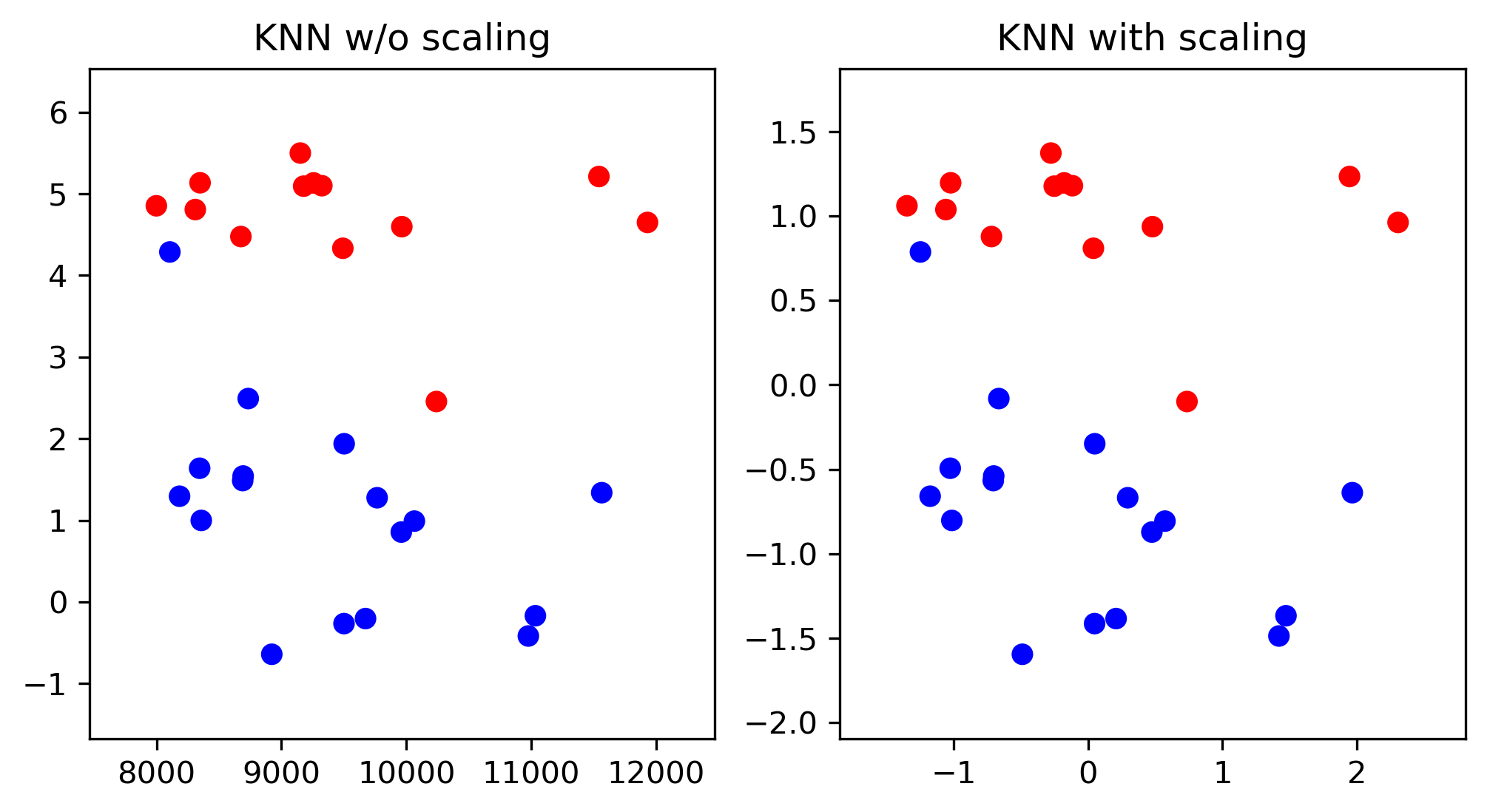
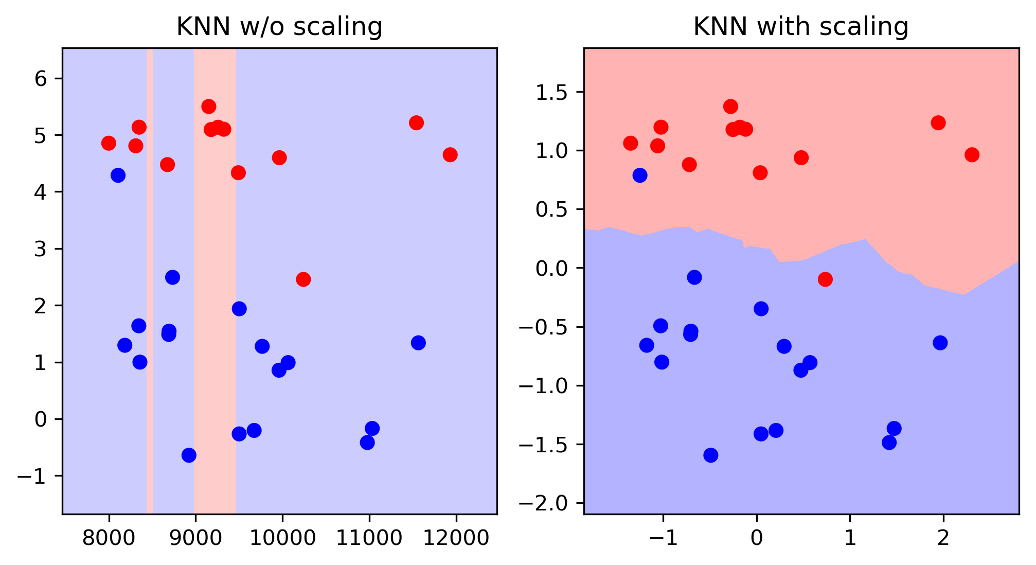
Importance of Scaling

Here’s an illustration why this is important using the min-max scaler. Left is the original data. Center is what happens when we fit on the training set and then transform the training and test set using this transformer. The data looks exactly the same, but the ticks changed. Now the data has a minimum of zero and a maximum of one on the training set. That’s not true for the test set, though. No particular range is ensured for the test-set. It could even be outside of 0 and 1. But the transformation is consistent with the transformation on the training set, so the data looks the same.

On the right you see what happens when you use the test-set minimum and maximum for scaling the test set. That’s what would happen if you’d fit again on the test set. Now the test set also has minimum at 0 and maximum at 1, but the data is totally distorted from what it was before. So don’t do that.

Scikit-Learn API

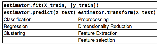
Shortcuts:

est.fit_transform(X) == est.fit(X).transform(X) (mostly)
est.fit_predict(X) == est.fit(X).predict(X) (mostly)

Here’s a summary of the scikit-learn methods. All models have a fit method which takes the training data X_train. If the model is supervised, such as our classification and regression models, they also take a y_train parameter. The scalers don’t use a y_train because they don’t use the labels at all – you could say they are unsupervised methods, but arguably they are not really learning methods at all. Models (also known as estimators in scikit-learn) to make a prediction of a target variable, you use the predict method, as in classification and regression. If you want to create a new representation of the data, a new kind of X, then you use the transform method, as we did with scaling. The transform method is also used for preprocessing, feature extraction and feature selection, which we’ll see later. All of these change X into some new form. There’s two important shortcuts. To fit an estimator and immediately transform the training data, you can use fit_transform. That’s often more efficient then using first fit and then transform. The same goes for fit_predict.

scores = cross_val_score(RidgeCV(), X_train, y_train, cv=10)
print2(np.mean(scores), np.std(scores))

(0.717, 0.125)

scores = cross_val_score(RidgeCV(), X_train_scaled, y_train, cv=10)
print2(np.mean(scores), np.std(scores))

(0.718, 0.127)

scores = cross_val_score(KNeighborsRegressor(), X_train, y_train, cv=10)
print2(np.mean(scores), np.std(scores))

(0.499, 0.146)

scores = cross_val_score(KNeighborsRegressor(), X_train_scaled, y_train, cv=10)
print2(np.mean(scores), np.std(scores))

(0.750, 0.106)

Preprocessing with Pipelines

A Common Error

print(X.shape)

(100, 10000)

# select most informative 5% of features
from sklearn.feature_selection import SelectPercentile, f_regression
select = SelectPercentile(score_func=f_regression, percentile=5)
select.fit(X, y)
X_selected = select.transform(X)
print(X_selected.shape)

(100, 500)

np.mean(cross_val_score(Ridge(), X_selected, y))

0.90

ridge = Ridge().fit(X_selected, y)
X_test_selected = select.transform(X_test)
ridge.score(X_test_selected, y_test)

-0.18

Leaking Information

# BAD!
select.fit(X, y)  # includes the cv test parts!
X_sel = select.transform(X)
scores = []
for train, test in cv.split(X, y):
    ridge = Ridge().fit(X_sel[train], y[train])
    score = ridge.score(X_sel[test], y[test])
    scores.append(score)

# GOOD!
scores = []
for train, test in cv.split(X, y):
    select.fit(X[train], y[train])
    X_sel_train = select.transform(X[train])
    ridge = Ridge().fit(X_sel_train, y[train])
    X_sel_test = select.transform(X[test])
    score = ridge.score(X_sel_test, y[test])
    scores.append(score)

Need to include preprocessing in cross-validation!

What we did was we trained the scaler on the training data, and then applied cross-validation to the scaled data. Tha’s what’s show on the left. The problem is that we use the information of all of the training data for scaling, so in particular the information in the test fold. This is also known as information leakage. If we apply our model to new data, this data will not have been used to do the scaling, so our cross-validation will give us a biased result that might be too optimistic.

On the right you can see how we should do it: we should only use the training part of the data to find the mean and standard deviation, even in cross-validation. That means that for each split in the cross-validation, we need to scale the data a bit differently. This basically means the scaling should happen inside the cross-validation loop, not outside.

In practice, estimating mean and standard deviation is quite robust and you will not see a big difference between the two methods. But for other preprocessing steps that we’ll see later, this might make a huge difference. So we should get it right from the start.

Leaking Information

Information leak:

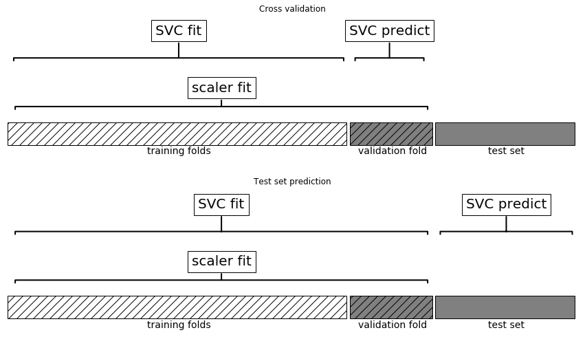
No information leak:

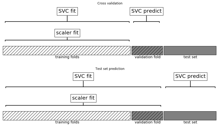
Need to include preprocessing in cross-validation!

X, y = boston.data, boston.target
X_train, X_test, y_train, y_test = \
	train_test_split(X, y, random_state=0)
scaler = StandardScaler()
scaler.fit(X_train)
X_train_scaled = scaler.transform(X_train)
ridge = Ridge().fit(X_train_scaled, y_train)

X_test_scaled = scaler.transform(X_test)
print2(ridge.score(X_test_scaled, y_test))

(0.635)

from sklearn.pipeline import make_pipeline
pipe = make_pipeline(StandardScaler(), Ridge())
pipe.fit(X_train, y_train)
print2(pipe.score(X_test, y_test))

(0.635)

Now I want to show you how to do preprocessing and crossvalidation right with scikit-learn.

At the top here you see the workflow for scaling the data and then applying ridge again. Fit the scaler on the training set, transform on the training set, fit ridge on the training set, transform the test set, and evaluate the model.

Because this is such a common pattern, scikit-learn has a tool to make this easier, the pipeline. The pipeline is an estimator that allows you to chain multiple transformations of the data before you apply a final model.

You can build a pipeline using the make_pipeline function. Just provide as parameters all the estimators. All but the last one need to have a transform method. Here we only have two steps: the standard scaler and ridge.

make_pipeline returns an estimator that does both steps at once. We can call fit on it to fit first the scaler and then ridge on the scaled data, and when we call score, it transforms the data and then evaluates the model.

Pipelines

Let’s dive a bit more into the pipeline. Here is an illustration of what happens with three steps, T1, T2 and Classifier. Imagine T1 to be a scaler and T2 to be any other transformation of the data.

If we call fit on this pipeline, it will first call fit on the first step with the input X. Then it will transform the input X to X1, and use X1 to fit the second step, T2. Then it will use T2 to transform the data from X1 to X2. Then it will fit the classifier on X2.

If we call predict on some data X’, say the test set, it will call transform on T1, creating X’1. Then it will use T2 to transform X’1 into X’2, and call the predict method of the classifier on X’2. This sounds a bit complicated, but it’s really just doing “the right thing” to apply multiple transformation steps.

Undoing our feature selection mistake

# BAD!
select.fit(X, y)  # includes the cv test parts!
X_sel = select.transform(X)
scores = []
for train, test in cv.split(X, y):
    ridge = Ridge().fit(X_sel[train], y[train])
    score = ridge.score(X_sel[test], y[test])
    scores.append(score)

Same as:

select.fit(X, y)
X_selected = select.transform(X, y)
np.mean(cross_val_score(Ridge(), X_selected, y))

0.90

# GOOD!
scores = []
for train, test in cv.split(X, y):
    select.fit(X[train], y[train])
    X_sel_train = select.transform(X[train])
    ridge = Ridge().fit(X_sel_train, y[train])
    X_sel_test = select.transform(X[test])
    score = ridge.score(X_sel_test, y[test])
    scores.append(score)

Same as:

pipe = make_pipeline(select, Ridge())
np.mean(cross_val_score(pipe, X, y))

-0.079

Naming Steps

from sklearn.pipeline import make_pipeline
knn_pipe = make_pipeline(StandardScaler(),
                         KNeighborsRegressor())
print(knn_pipe)

Pipeline(steps=[('standardscaler', StandardScaler()),
                ('kneighborsregressor', KNeighborsRegressor())])

from sklearn.pipeline import Pipeline
pipe = Pipeline((("scaler", StandardScaler()),
                 ("regressor", KNeighborsRegressor)))

Pipeline and GridSearchCV

knn_pipe = make_pipeline(StandardScaler(),
                         KNeighborsRegressor())
param_grid = \
    {'kneighborsregressor__n_neighbors': range(1, 10)}
grid = GridSearchCV(knn_pipe, param_grid, cv=10)
grid.fit(X_train, y_train)
print(grid.best_params_)
print2(grid.score(X_test, y_test))

{'kneighborsregressor__n_neighbors': 7}
(0.600)

These names are important for using pipelines with gridsearch. Recall that for using GridSearchCV you need to specify a parameter grid as a dictionary, where the keys are the parameter names. If you are using a pipeline inside GridSearchCV, you need to specify not only the parameter name, but also the step name – because multiple steps could have a parameter with the same name.

The way to do this is to use the stepname, then two underscores, and then the parameter name, as the key for the param_grid dictionary.

You can see that the bestparams will have this same format.

This way you can tune the parameters of all steps in a pipeline at once!

And you don’t have to worry about leaking information, since all transformations are contained in the pipeline.

You should always use pipelines for preprocessing. Not only does it make your code shorter, it also makes it less likely that you have bugs.

Going wild with Pipelines

from sklearn.datasets import load_diabetes
diabetes = load_diabetes()
X_train, X_test, y_train, y_test = train_test_split(
    diabetes.data, diabetes.target, random_state=0)
from sklearn.preprocessing import PolynomialFeatures
pipe = make_pipeline(
    StandardScaler(),
    PolynomialFeatures(),
    Ridge())
param_grid = {'polynomialfeatures__degree': [1, 2, 3],
              'ridge__alpha': [0.001, 0.01, 0.1, 1, 10, 100]}
grid = GridSearchCV(pipe, param_grid=param_grid,
                    n_jobs=-1, return_train_score=True)
grid.fit(X_train, y_train)

Wilder

pipe = Pipeline([('scaler', StandardScaler()),
                 ('regressor', Ridge())])
param_grid = {'scaler': [StandardScaler(), MinMaxScaler(),
                         'passthrough'],
              'regressor': [Ridge(), Lasso()],
              'regressor__alpha': np.logspace(-3, 3, 7)}
grid = GridSearchCV(pipe, param_grid)
grid.fit(X_train, y_train)
grid.score(X_test, y_test)

Wildest

from sklearn.tree import DecisionTreeRegressor
pipe = Pipeline([('scaler', StandardScaler()),
                 ('regressor', Ridge())])
# check out searchgrid for more convenience
param_grid = [{'regressor': [DecisionTreeRegressor()],
               'regressor__max_depth': [2, 3, 4],
               'scaler': ['passthrough']},
              {'regressor': [Ridge()],
               'regressor__alpha': [0.1, 1],
               'scaler': [StandardScaler(), MinMaxScaler(),
                          'passthrough']}
             ]
grid = GridSearchCV(pipe, param_grid)
grid.fit(X_train, y_train)

Feature Distributions

Transformed Features

Transformed Histograms

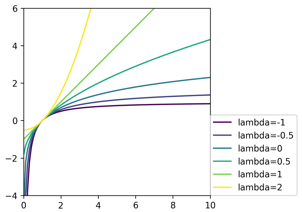
Power Transformations

\begin{equation} bc_\lambda(x) = \begin{cases} \frac{x^\lambda - 1}{\lambda} & \text{ if $\lambda \ne 0$}\\ \log(x) & \text{ if $\lambda =0$}\\ \end{cases} \end{equation}

Only applicable for positive $x$!

from sklearn.preprocessing import PowerTransformer
pt = PowerTransformer(method='box-cox')
# for any data: Yeo-Johnson
pt.fit(X)

Box-Cox on Boston

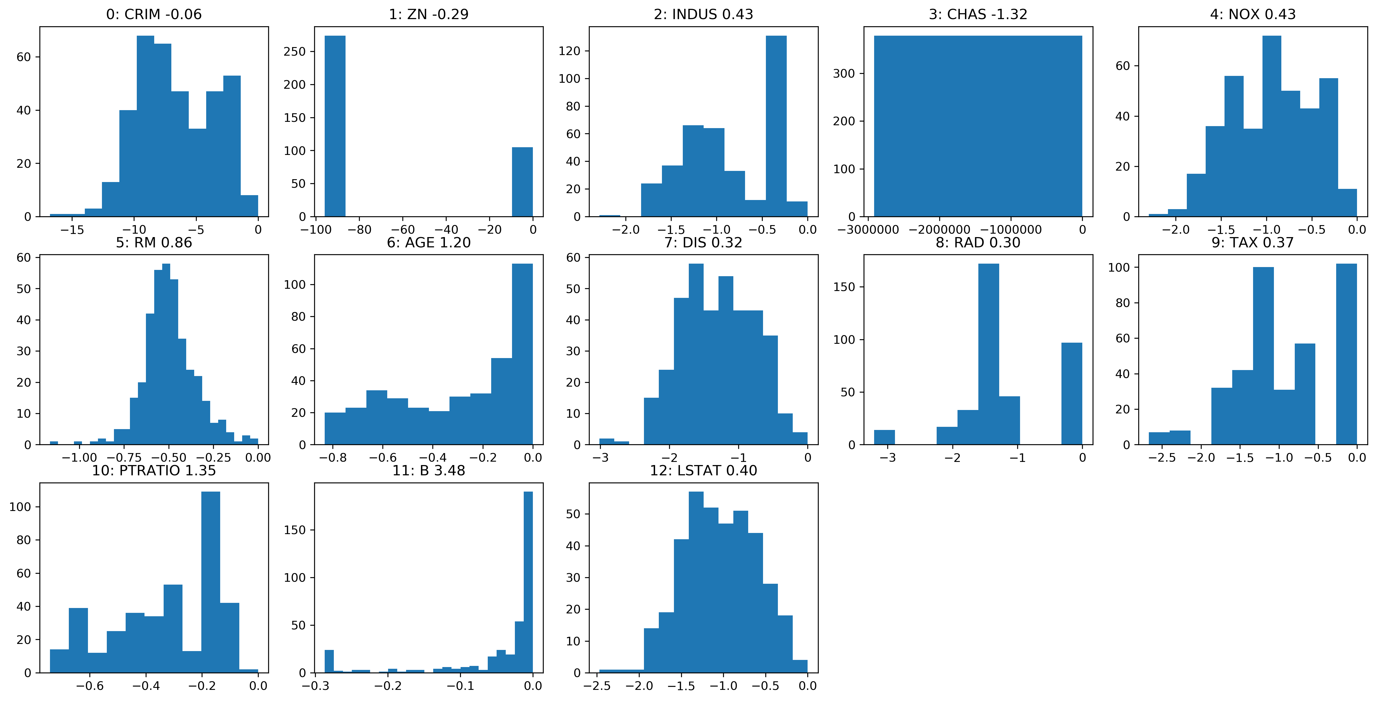
Before

After

Box-Cox Scatter

Before

After

Categorical Variables

df = pd.DataFrame({
    'boro': ['Manhattan', 'Queens', 'Manhattan', 'Brooklyn', 'Brooklyn', 'Bronx'],
    'salary': [103, 89, 142, 54, 63, 219],
    'vegan': ['No', 'No','No','Yes', 'Yes', 'No']})

	boro	salary	vegan
0	Manhattan	103	No
1	Queens	89	No
2	Manhattan	142	No
3	Brooklyn	54	Yes
4	Brooklyn	63	Yes
5	Bronx	219	No

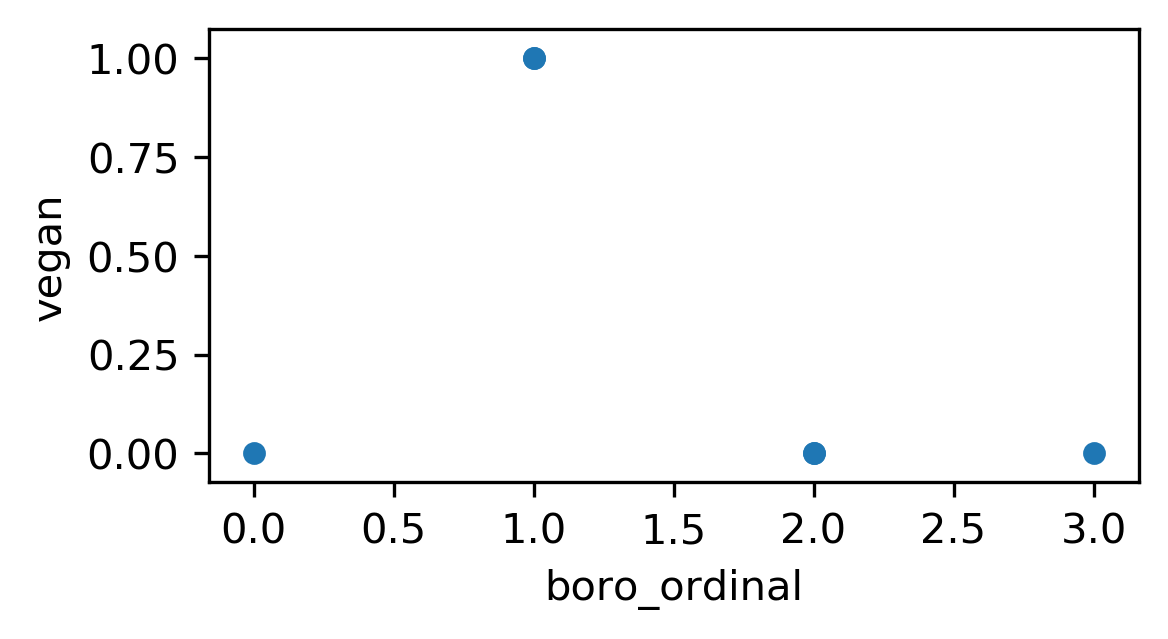
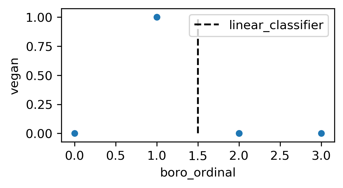
Ordinal Encoding

df['boro_ordinal'] = df.boro.astype("category").cat.codes

	boro	salary	vegan	boro_ordinal
0	Manhattan	103	No	2
1	Queens	89	No	3
2	Manhattan	142	No	2
3	Brooklyn	54	Yes	1
4	Brooklyn	63	Yes	1
5	Bronx	219	No	0

One-Hot (Dummy) Encoding

	boro	salary	vegan
0	Manhattan	103	No
1	Queens	89	No
2	Manhattan	142	No
3	Brooklyn	54	Yes
4	Brooklyn	63	Yes
5	Bronx	219	No

pd.get_dummies(df)

	salary	boro_Bronx	boro_Brooklyn	boro_Manhattan	boro_Queens	vegan_No	vegan_Yes
0	103	0	0	1	0	1	0
1	89	0	0	0	1	1	0
2	142	0	0	1	0	1	0
3	54	0	1	0	0	0	1
4	63	0	1	0	0	0	1
5	219	1	0	0	0	1	0

Instead, we add one new feature for each category,

And that feature encodes whether a sample belongs to this category or not.

That’s called a one-hot encoding, because only one of the three features in this example is active at a time.

You could actually get away with n-1 features, but in machine learning that usually doesn’t matter

One way to do is with Pandas. Here I have an example of a data frame where I have the boroughs of New York as a categorical variable and variable saying whether they are vegan. One to get the dummies is to get dummies on this data frame. This will create new columns, it will actually replace borough column by four columns that correspond to the four different values. The get_dummies applies transformation to all columns that have a dtype that's either object or categorical.

In this case we didn't actually want to transform the target variable vegan.

One-Hot (Dummy) Encoding

	boro	salary	vegan
0	Manhattan	103	No
1	Queens	89	No
2	Manhattan	142	No
3	Brooklyn	54	Yes
4	Brooklyn	63	Yes
5	Bronx	219	No

pd.get_dummies(df, columns=['boro'])

	salary	vegan	boro_Bronx	boro_Brooklyn	boro_Manhattan	boro_Queens
0	103	No	0	0	1	0
1	89	No	0	0	0	1
2	142	No	0	0	1	0
3	54	Yes	0	1	0	0
4	63	Yes	0	1	0	0
5	219	No	1	0	0	0

One-Hot (Dummy) Encoding

	boro	salary	vegan
0	Manhattan	103	No
1	Queens	89	No
2	Manhattan	142	No
3	Brooklyn	54	Yes
4	Brooklyn	63	Yes
5	Bronx	219	No

pd.get_dummies(df_ordinal, columns=['boro'])

	salary	vegan	boro_0	boro_1	boro_2	boro_3
0	103	No	0	0	1	0
1	89	No	0	0	0	1
2	142	No	0	0	1	0
3	54	Yes	0	1	0	0
4	63	Yes	0	1	0	0
5	219	No	1	0	0	0

df = pd.DataFrame({
    'boro': ['Manhattan', 'Queens', 'Manhattan',
             'Brooklyn', 'Brooklyn', 'Bronx'],
    'salary': [103, 89, 142, 54, 63, 219],
    'vegan': ['No', 'No','No','Yes', 'Yes', 'No']})
df_dummies = pd.get_dummies(df, columns=['boro'])

	salary	vegan	boro_Bronx	boro_Brooklyn	boro_Manhattan	boro_Queens
0	103	No	0	0	1	0
1	89	No	0	0	0	1
2	142	No	0	0	1	0
3	54	Yes	0	1	0	0
4	63	Yes	0	1	0	0
5	219	No	1	0	0	0

df = pd.DataFrame({
    'boro': ['Brooklyn', 'Manhattan', 'Brooklyn',
             'Queens', 'Brooklyn', 'Staten Island'],
    'salary': [61, 146, 142, 212, 98, 47],
    'vegan': ['Yes', 'No','Yes','No', 'Yes', 'No']})
df_dummies = pd.get_dummies(df, columns=['boro'])

	salary	vegan	boro_Brooklyn	boro_Manhattan	boro_Queens	boro_Staten Island
0	61	Yes	1	0	0	0
1	146	No	0	1	0	0
2	142	Yes	1	0	0	0
3	212	No	0	0	1	0
4	98	Yes	1	0	0	0
5	47	No	0	0	0	1

Pandas Categorial Columns

df = pd.DataFrame({
    'boro': ['Manhattan', 'Queens', 'Manhattan',
             'Brooklyn', 'Brooklyn', 'Bronx'],
    'salary': [103, 89, 142, 54, 63, 219],
    'vegan': ['No', 'No','No','Yes', 'Yes', 'No']})
df['boro'] = pd.Categorical(df.boro,
                            categories=['Manhattan', 'Queens', 'Brooklyn',
                                        'Bronx', 'Staten Island'])
pd.get_dummies(df, columns=['boro'])

	salary	vegan	boro_Manhattan	boro_Queens	boro_Brooklyn	boro_Bronx
0	103	No	1	0	0	0
1	89	No	0	1	0	0
2	142	No	1	0	0	0
3	54	Yes	0	0	1	0
4	63	Yes	0	0	1	0
5	219	No	0	0	0	1

The way to fix this is by using Pandas categorical types. Since we know what the boroughs of Manhattan are, we can create Pandas categorical dtype, we can create this categorical dtype with the categories Manhattan, Queens, Brooklyn, Bronx, and Staten Island. So now I have my column here and I'm going to convert it to a categorical dtype. So now it will not actually store the strings. It will just internally store zero to four, and it will also store what are the possible values. If a call get_dummies it will use all the possible values and for each of the possible values it will create a column. Even though Staten Island has not appeared in my dataset, it will still make a column for Staten Island. If I fix this categorical dtype I can apply it to the training and test data set and that'll make sure all the columns are always the same no matter what are the values are actually in the data set.

`OneHotEncoder`

from sklearn.preprocessing import OneHotEncoder
df = pd.DataFrame({'salary': [103, 89, 142, 54, 63, 219],
                   'boro': ['Manhattan', 'Queens', 'Manhattan',
                            'Brooklyn', 'Brooklyn', 'Bronx']})
ce = OneHotEncoder().fit(df)
print(ce.transform(df).toarray())

[[0. 0. 0. 1. 0. 0. 0. 0. 1. 0.]
 [0. 0. 1. 0. 0. 0. 0. 0. 0. 1.]
 [0. 0. 0. 0. 1. 0. 0. 0. 1. 0.]
 [1. 0. 0. 0. 0. 0. 0. 1. 0. 0.]
 [0. 1. 0. 0. 0. 0. 0. 1. 0. 0.]
 [0. 0. 0. 0. 0. 1. 1. 0. 0. 0.]]

always transforms all columns!

`OneHotEncoder` + `ColumnTransformer`

categorical = df.dtypes == object
preprocess = make_column_transformer(
    (StandardScaler(), ~categorical),
    (OneHotEncoder(), categorical))
model = make_pipeline(preprocess, LogisticRegression())
model

Pipeline(steps=[('columntransformer',
                 ColumnTransformer(transformers=[('standardscaler',
                                                  StandardScaler(),
                                                  salary     True
boro      False
dtype: bool),
                                                 ('onehotencoder',
                                                  OneHotEncoder(),
                                                  salary    False
boro       True
dtype: bool)])),
                ('logisticregression', LogisticRegression())])

Dummy variables and colinearity

One-hot is redundant (last one is 1 – sum of others)
Can introduce co-linearity
Can drop one
Choice which one matters for penalized models
Keeping all can make the model more interpretable

Models Supporting Discrete Features

In principle:
- All tree-based models, naive Bayes
In scikit-learn:
- Some Naive Bayes classifiers.
In scikit-learn "soon":
- Decision trees, random forests, gradient boosting

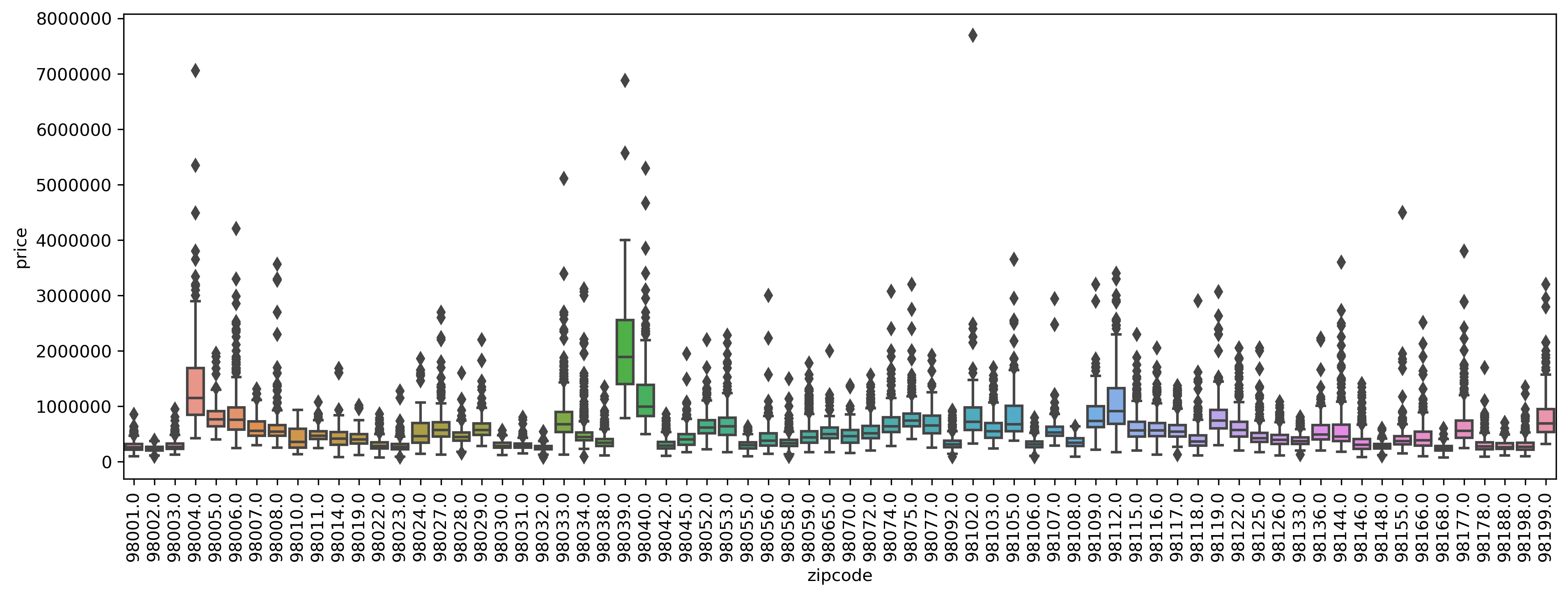
Target Encoding (Impact Encoding)

For high cardinality categorical features
Instead of 70 one-hot variables, one “response encoded” variable.
For regression: "average price in zip code”
Binary classification: “building in this zip code have a likelihood p for class 1”
Multiclass: One feature per class – probability distribution

So there's also another way to encode categorical variables that is often used, I like to call it target-Based Encoding. It's basically for very high cardinality categorical features. For example, if you have categorical feature it's all US states and you don't have a lot of samples or if you have categorical features that's all US zip codes, if you have all different things, you don't want to do One Hot Encoding. So you get 50 new features, which if you don't have a lot of data would be a lot of features. So instead, you can use one single variable, it basically encodes the response. So for regression, it would be people in this state have an average response of that. Obviously you don't want to do this on the test set basically or you want to do this on the whole dataset for each level of the categorical variable, you want to find out what is the mean response and just use this as the future value. So you get one single future. For binary classification, you can just use the fraction of people that are classified as Class One. For multi-class, you usually do the percentage or fraction of people in each of the classes. So in multi-class, you get one new feature per class and you count for each state how many people in this state are classified for each of them.

More encodings for categorical features:

http://contrib.scikit-learn.org/categorical-encoding/

Load data, include ZIP code

from sklearn.datasets import fetch_openml
data = fetch_openml("house_sales", as_frame=True)
X = data.frame.drop(['date', 'price'], axis=1)
y = data.frame['price']
X_train, X_test, y_train, y_test = train_test_split(X, y)
X_train.columns

Index(['bedrooms', 'bathrooms', 'sqft_living', 'sqft_lot', 'floors',
       'waterfront', 'view', 'condition', 'grade', 'sqft_above',
       'sqft_basement', 'yr_built', 'yr_renovated', 'zipcode', 'lat', 'long',
       'sqft_living15', 'sqft_lot15'],
      dtype='object')

X_train.head()

	bedrooms	bathrooms	sqft_living	sqft_lot	floors	...	zipcode	lat	long	sqft_living15	sqft_lot15
5945	4.0	2.25	1810.0	9240.0	2.0	...	98055.0	47.4362	-122.187	1660.0	9240.0
8423	3.0	2.50	1600.0	2788.0	2.0	...	98031.0	47.4034	-122.187	1720.0	3605.0
13488	4.0	2.50	1720.0	8638.0	2.0	...	98003.0	47.2704	-122.313	1870.0	7455.0
20731	2.0	2.25	1240.0	705.0	2.0	...	98027.0	47.5321	-122.073	1240.0	750.0
2358	3.0	2.00	1280.0	13356.0	1.0	...	98042.0	47.3715	-122.074	1590.0	8071.0

import category_encoders as ce
te = ce.TargetEncoder(cols='zipcode').fit(X_train,  y_train)
te.transform(X_train).head()

	bedrooms	bathrooms	sqft_living	sqft_lot	floors	...	zipcode	lat	long	sqft_living15	sqft_lot15
5945	4.0	2.25	1810.0	9240.0	2.0	...	305061.113861	47.4362	-122.187	1660.0	9240.0
8423	3.0	2.50	1600.0	2788.0	2.0	...	303052.073892	47.4034	-122.187	1720.0	3605.0
13488	4.0	2.50	1720.0	8638.0	2.0	...	290589.201970	47.2704	-122.313	1870.0	7455.0
20731	2.0	2.25	1240.0	705.0	2.0	...	618687.511785	47.5321	-122.073	1240.0	750.0
2358	3.0	2.00	1280.0	13356.0	1.0	...	314250.081967	47.3715	-122.074	1590.0	8071.0

y_train.groupby(X_train.zipcode).mean()[X_train.head().zipcode]

zipcode
98055.0    305061.113861
98031.0    303052.073892
98003.0    290589.201970
98027.0    618687.511785
98042.0    314250.081967
Name: price, dtype: float64

Results

X = data.frame.drop(['date', 'price', 'zipcode'], axis=1)
scores = cross_val_score(Ridge(), X, y)
print(f"{np.mean(scores):.2f}")

0.69

from sklearn.compose import make_column_transformer
from sklearn.preprocessing import OneHotEncoder
X = data.frame.drop(['date', 'price'], axis=1)
ct = make_column_transformer((OneHotEncoder(), ['zipcode']), remainder='passthrough')
pipe_ohe = make_pipeline(ct, Ridge())
scores = cross_val_score(pipe_ohe, X, y)
print(f"{np.mean(scores):.2f}")

0.53

pipe_target = make_pipeline(ce.TargetEncoder(cols='zipcode'), Ridge())
scores = cross_val_score(pipe_target, X, y)
print(f"{np.mean(scores):.2f}")

0.79

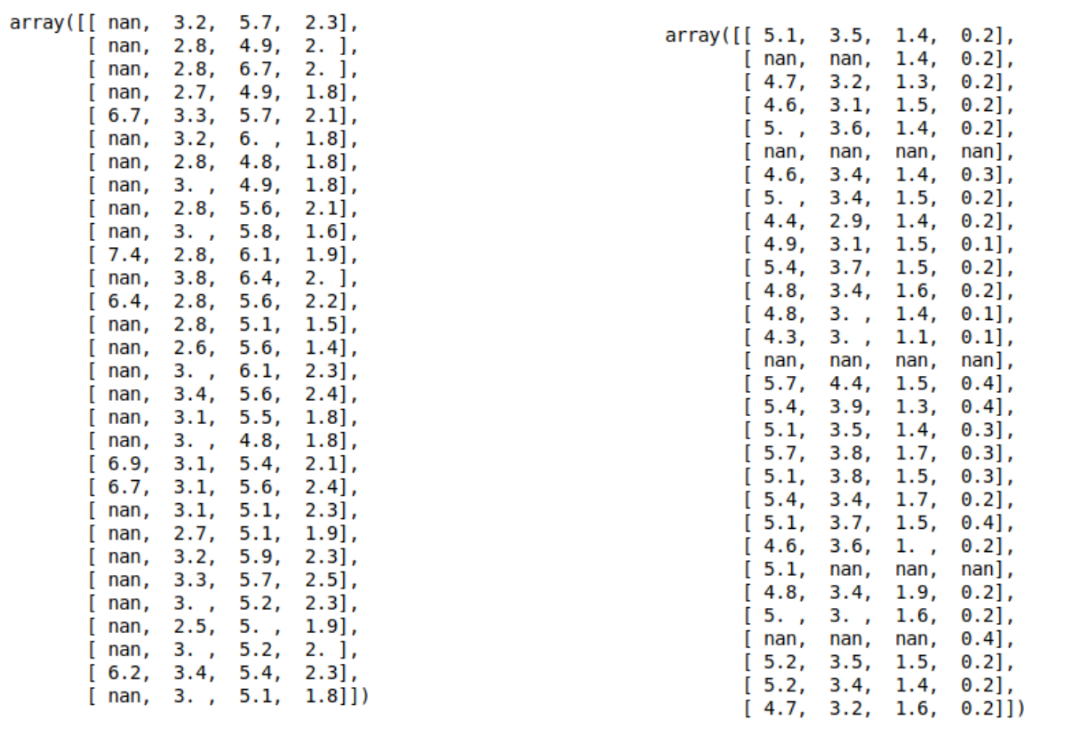
Imputation

Dealing with missing values

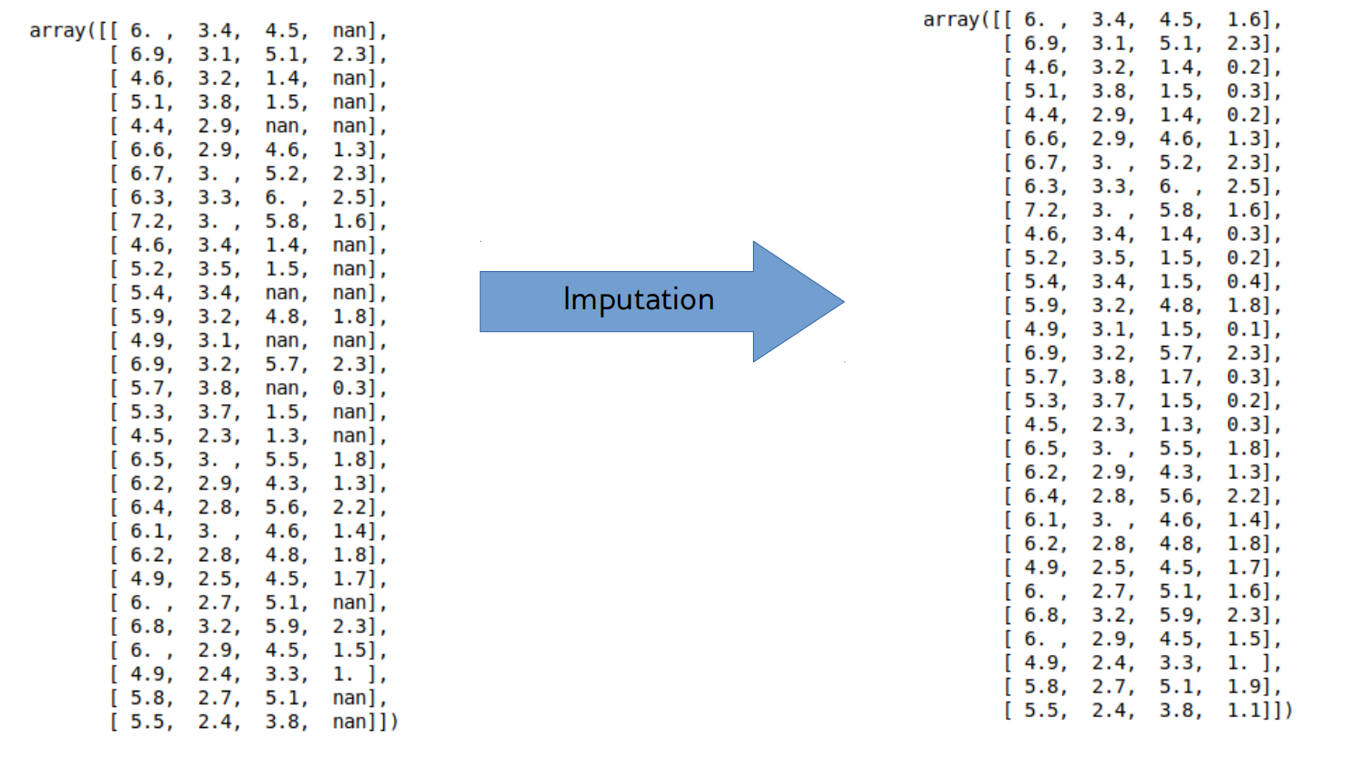
Imputation Methods

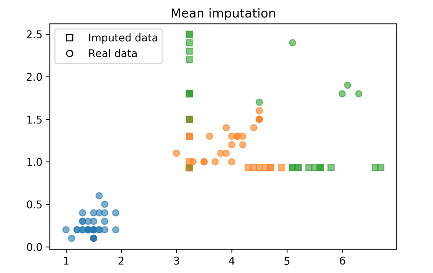
Mean/Median
kNN
Regression models
Probabilistic models

Baseline: Dropping Columns

from sklearn.linear_model import LogisticRegressionCV
X_train, X_test, y_train, y_test = \
    train_test_split(X_, y, stratify=y)
nan_columns = np.any(np.isnan(X_train), axis=0)
X_drop_columns = X_train[:, ~nan_columns]
scores = cross_val_score(LogisticRegressionCV(v=5), 
                         X_drop_columns, y_train, cv=10)
np.mean(scores)

0.772

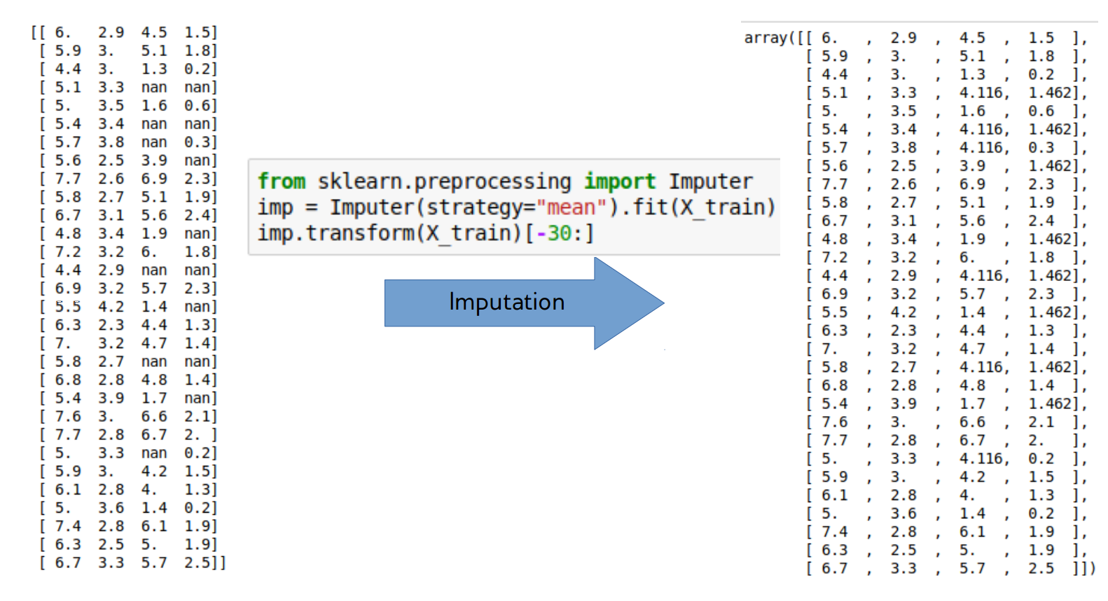
Mean and Median

from sklearn.pipeline import make_pipeline
from sklearn.preprocessing import StandardScalar
nan_columns = np.any(np.isnan(X_train), axis = 0)
X_drop_columns = X_train[:,~nan_columns]
logreg = make_pipeline(StandardScalar(),
                       LogisticRegression())
scores = cross_val_score(logreg, X_drop_columns,
                         y_train, cv = 10)
print(np.mean(scores))

mean_pipe = make_pipeline(SimpleImputer(), StandardScalar(),
                          LogisticRegression())
scores = cross_val_score(mean_pipe, X_train, y_train, cv=10)
print(np.mean(scores))

0.794
0.729

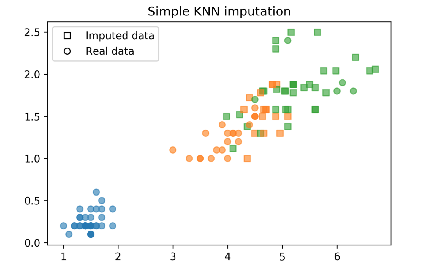
kNN Imputation

Find k nearest neighbors that have non-missing values.
Fill in all missing values using the average of the neighbors.

sklearn.impute import KNNImputer
imputer = KNNImputer(n_neighbors=2)
imputer.fit_transform(X)

kNN Imputation Code

distances = np.zeros((X_train.shape[0], X_train.shape[0]))
for i, x1 in enumerate(X_train):
    for j, x2 in enumerate(X_train):
        dist = (x1 - x2) ** 2
        nan_mask = np.isnan(dist)
        distances[i, j] = dist[~nan_mask].mean() * X_train.shape[1]
neighbors = np.argsort(distances, axis=1)[:, 1:]
n_neighbors = 3
X_train_knn = X_train.copy()
for feature in range(X_train.shape[1]):
    has_missing_value = np.isnan(X_train[:, feature])
    for row in np.where(has_missing_value)[0]:
        neighbor_features = X_train[neighbors[row], feature]
        non_nan_neighbors = \
            neighbor_features[~np.isnan(neighbor_features)]
        X_train_knn[row, feature] = \
            non_nan_neighbors[:n_neighbors].mean()

kNN Imputation Plot

scores = cross_val_score(logreg, X_train_knn, y_train, cv=10)
np.mean(scores)

0.849

Model-Driven Imputation

Train regression model for missing values
Possibly iterate: retrain after filling in
Very flexible!

Model-driven imputation with RF

rf = RandomForestRegressor(n_estimators=100)
X_imputed = X_train.copy()
for i in range(10):
    last = X_imputed.copy()
    for feature in range(X_train.shape[1]):
        inds_not_f = np.arange(X_train.shape[1])
        inds_not_f = inds_not_f[inds_not_f != feature]
        f_missing = np.isnan(X_train[:, feature])
        rf.fit(X_imputed[~f_missing][:, inds_not_f],
               X_train[~f_missing, feature])
        X_imputed[f_missing, feature] = rf.predict(
            X_imputed[f_missing][:, inds_not_f])
    if (np.linalg.norm(last - X_imputed)) < .5:
        break
scores = cross_val_score(logreg, X_imputed, y_train, cv=10)
np.mean(scores)

0.855

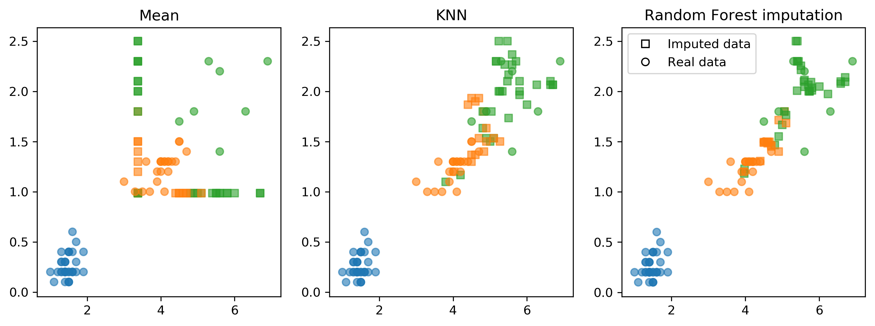
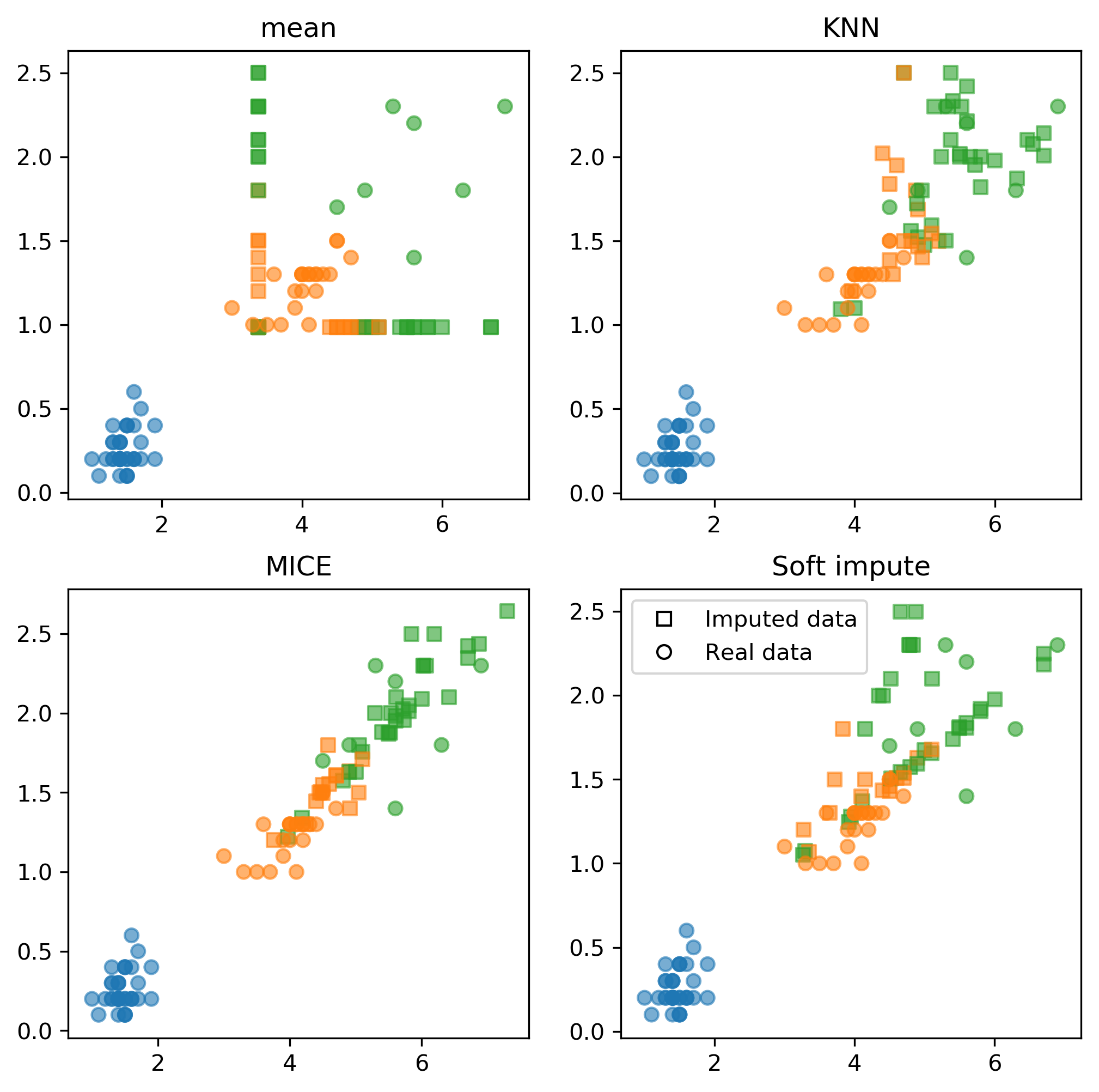
Imputation Method Comparison

Fancyimpute

!pip install fancyimpute
sklearn's IterativeImputer can work well..
fancyimpute provides fancier features

Applying `fancyimpute`

from fancyimpute import IterativeImputer
imputer = IterativeImputer(n_iter=5)
X_complete = imputer.fit_transform(X_train)

scores = cross_val_score(logreg, X_train_fancy_mice, 
                         y_train, cv=10)
np.mean(scores)

0.866

	salary	vegan	boro_Brooklyn	boro_Manhattan	boro_Queens	boro_Staten Island
0	61	Yes	1	0	0	0
1	146	No	0	1	0	0
2	142	Yes	1	0	0	0
3	212	No	0	0	1	0
4	98	Yes	1	0	0	0
5	47	No	0	0	0	1

	salary	vegan	boro_Manhattan	boro_Queens	boro_Brooklyn	boro_Bronx
0	103	No	1	0	0	0
1	89	No	0	1	0	0
2	142	No	1	0	0	0
3	54	Yes	0	0	1	0
4	63	Yes	0	0	1	0
5	219	No	0	0	0	1

	salary	vegan	boro_Brooklyn	boro_Manhattan	boro_Queens	boro_Staten Island
0	61	Yes	1	0	0	0
1	146	No	0	1	0	0
2	142	Yes	1	0	0	0
3	212	No	0	0	1	0
4	98	Yes	1	0	0	0
5	47	No	0	0	0	1

	salary	vegan	boro_Manhattan	boro_Queens	boro_Brooklyn	boro_Bronx
0	103	No	1	0	0	0
1	89	No	0	1	0	0
2	142	No	1	0	0	0
3	54	Yes	0	0	1	0
4	63	Yes	0	0	1	0
5	219	No	0	0	0	1

Preprocessing

09/09/2022

Robert Utterback (based on slides by Andreas Muller)

Preprocessing

Scaling

Scaling and Distances

Scaling and Distances

Ways to Scale Data

Sparse Data

Standard Scaler Example

Importance of Scaling

Scikit-Learn API

Preprocessing with Pipelines

A Common Error

Leaking Information

Leaking Information

Pipelines

Undoing our feature selection mistake

Naming Steps

Pipeline and GridSearchCV

Going wild with Pipelines

Wilder

Wildest

Feature Distributions

Transformed Features

Transformed Histograms

Power Transformations

Box-Cox on Boston

Box-Cox Scatter

Categorical Variables

Categorical Variables

Ordinal Encoding

One-Hot (Dummy) Encoding

One-Hot (Dummy) Encoding

One-Hot (Dummy) Encoding

Pandas Categorial Columns

OneHotEncoder

OneHotEncoder + ColumnTransformer

Dummy variables and colinearity

Models Supporting Discrete Features

Target Encoding (Impact Encoding)

Target Encoding (Impact Encoding)

More encodings for categorical features:

Load data, include ZIP code

Results

Imputation

Dealing with missing values

Imputation Methods

Baseline: Dropping Columns

Mean and Median

kNN Imputation

kNN Imputation Code

kNN Imputation Plot

Model-Driven Imputation

Model-driven imputation with RF

Imputation Method Comparison

Fancyimpute

Applying fancyimpute

`OneHotEncoder`

`OneHotEncoder` + `ColumnTransformer`

Applying `fancyimpute`

	salary	vegan	boro_Brooklyn	boro_Manhattan	boro_Queens	boro_Staten Island
0	61	Yes	1	0	0	0
1	146	No	0	1	0	0
2	142	Yes	1	0	0	0
3	212	No	0	0	1	0
4	98	Yes	1	0	0	0
5	47	No	0	0	0	1

	salary	vegan	boro_Manhattan	boro_Queens	boro_Brooklyn	boro_Bronx
0	103	No	1	0	0	0
1	89	No	0	1	0	0
2	142	No	1	0	0	0
3	54	Yes	0	0	1	0
4	63	Yes	0	0	1	0
5	219	No	0	0	0	1